This assumption is often presented as demanding complete independence between the errors, and from time to time I will use the concept of independence as a convenient shorthand, but we may relax this assumption to simply require the errors be uncorrelated, and all of our useful OLS results will still hold.
When the errors are correlated, we say that the data show serial correlation, which is also called autocorrelation.
Categories and illustrations of serial correlation
Most of the literature on serial correlation describes data with an obvious time series nature, such as daily market prices or hourly transaction totals. However, many datasets will show serial correlation even if they are completely cross-sectional, that is, gathered all at the same time:
Say that I administer a test to college students in five different classrooms. When I collate and enter the data, I will likely enter all the grades from one section, followed by a second, and a third, etc. Within each classroom, there might be unique factors (noise and light levels, teacher attributes, reasons why that time slot worked best for the students, etc.) which correlate errors within the same classroom.
Say that I reorder the dataset by student ID number. However, the student ID number might be a function of when they were first entered into the school’s IT systems. This in turn would be correlated with factors such cohort/graduation year, or whether a student was accepted through early admission or accepted late from the waitlist, which may also be correlated with educational outcomes.
Say that I reorder the dataset by student’s last name. However, last names starting with certain letters are more common in some countries than others, so once again we might observe some correlation between nearby observations, corresponding to linguistic and cultural similarities between the students.
You will note that the serial correlation in these examples has no real time series component but results instead from how we order the observations in our sample. As we shall see, this type of serial correlation does not always pose a problem for our analyses.
The more classic type of serial correlation results from data gathered regularly across a time interval, such as daily stock market prices. Using \(t\) to subscript the data instead of our customary \(i\), consider an error process which is itself a combination of the previous observation and a separate IID-normal error term:
Together, these two models become a regression with an “AR1” (first-order autocorrelation) error process, and when the model is estimated from a sample of data, we would expect to find serial correlation among the residuals, which are estimators for \(\varepsilon_t\). When the correlation parameter \(\rho\) is large and positive, the residuals resemble a random walk; when \(\rho\) is large and negative, the residuals will swing wildly from one residual to the next:
Code
set.seed(1860)par(mfrow=c(1,3))plot(arima.sim(model=list(ar=0.8),n=50),main=expression(paste('Autocorrelation of ',rho ==0.8)),ylim=c(-3,3),ylab='Residual')abline(h=0,lwd=2,lty=2,col='grey50')plot(arima.sim(model=list(ar=0.0),n=50),ylim=c(-3,3),main='No autocorrelation',ylab='Residual')
Warning in min(Mod(polyroot(c(1, -model$ar)))): no non-missing arguments to
min; returning Inf
Code
abline(h=0,lwd=2,lty=2,col='grey50')plot(arima.sim(model=list(ar=-0.8),n=50),main=expression(paste('Autocorrelation of ',rho ==-0.8)),ylim=c(-3,3),ylab='Residual')abline(h=0,lwd=2,lty=2,col='grey50')
Illustrations of positive and negative autocorrelation
Notice that each residual, if uncorrelated, should have an independent 50-50 chance of being either positive or negative. The probability of observing roughly 25 positive residuals in a row (in the leftmost plot above) would normally approach zero. Likewise, the probability of always observing a sign change from one residual to the next (in the rightmost plot above) should be near zero, just as it would be unusual to observe a sequence of coin flips HTHTHTHTHTHTHTH… By contrast, in the middle plot above, note that the next residual in a sequence has a roughly 50% chance of sharing the sign of the previous residual. In uncorrelated residuals, the past should not predict the present!
Consequences of serial correlation
Let’s consider three separate causes of serial correlation:
In some cases, serial correlation can be ignored without much consequence. When the data aren’t actually from a time series, and the serial correlation comes instead from an arbitrary ordering of the rows, and especially if the model will not be used for out-of-sample prediction, then mild or moderate serial correlation may be disregarded. In fact, for all but the most sensitive applications, a mild amount of serial correlation (say, \(|\rho| \le 0.1\)) may be disregarded, since the regression model almost surely has larger challenges elsewhere.
When the data instead shows true time series behavior, the presence of any amount of serial correlation begins to affect the model conclusions. Although “true” serial correlation does not bias the betas, it does distort many of the other model characteristics: the significance and standard errors of the betas, the estimated error variance, confidence intervals for predictions and mean responses, etc. Serial correlation also means the OLS model is no longer consistent, an estimation term meaning that the model estimators smoothly converge on the true parameters with larger and larger sample sizes.
Finally, when the serial correlation comes from omitted variables, we might say instead that the model is misspecified and that the serial correlation is simply a symptom of the misspecification, rather than a property of the data’s generating process. In such circumstances, the estimates of the betas may no longer be reliable, as the omitted variables could easily bias the regression results!
Identifying serial correlation
As with the discussion of Heteroskedasticity, there are two principal ways to identify serial correlation: examining plots of the data, and conducting hypothesis tests.
Diagnostic plots
A simple ordered plot of the residuals (like those above) will sometimes provide enough evidence to spark suspicion. However, the human eye is not very adept at distinguishing mild to moderate amounts of serial correlation.
Another way to notice autocorrelation is to plot the residuals against their own lagged values. For example, if your regression contains 100 residuals, plot the paired points \((e_1,e_2), (e_2,e_3), \ldots, (e_{99},e_{100})\). In cases of strong serial correlation you will see a linear trend to the data. However, even here the human eye can easily mislead us:
Code
set.seed(1833)par(mfrow=c(1,2))tmp <-arima.sim(model=list(ar=0.8),n=100)plot(tmp[1:99],tmp[2:100],main=expression(paste('Autocorrelation of ',rho ==0.8)),xlab='Previous Residual',ylab='Current Residual')tmp <-arima.sim(model=list(ar=-.15),n=100)plot(tmp[1:99],tmp[2:100],main=expression(paste('Autocorrelation of ',rho ==-0.15)),xlab='Previous Residual',ylab='Current Residual')
Plots of the residuals vs their own lagged values
As you can see above, strong positive autocorrelation leaves a clear trend in the lagged residuals, while weaker (but still substantial) negative correlation shows almost no evidence of a linear trend.
The best way to spot serial correlation is not to stare at the raw data, but to specifically plot the correlations of the residuals with its past values. This type of plot is known as an autocorrelation function (ACF) plot, and it can reveal not just first-order correlation, but also seasonality in the data beyond the first lag:1
Code
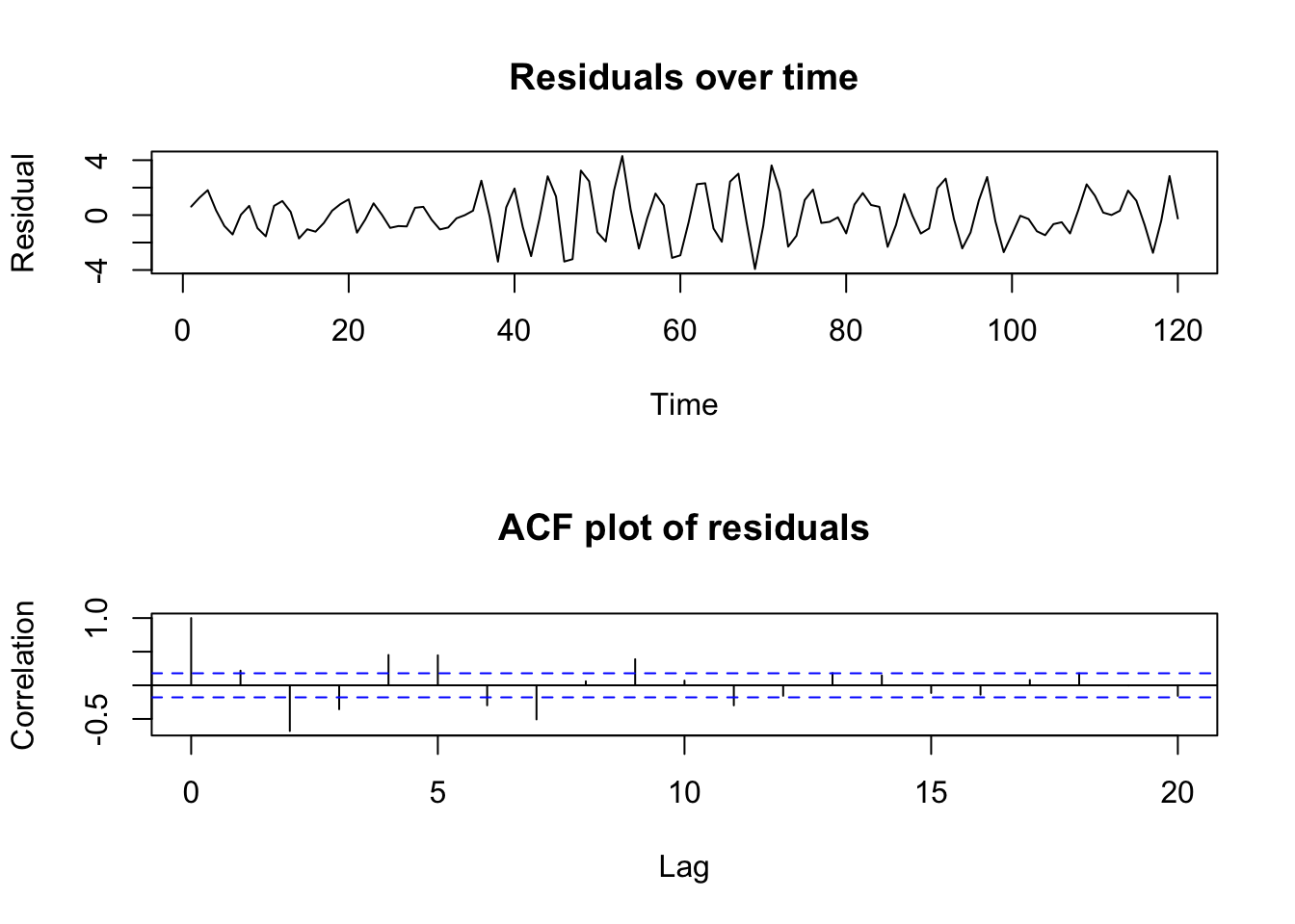
set.seed(1933)par(mfrow=c(2,1))tmp <-arima.sim(model=list(ar=c(0.4,-0.8),order=c(2,0,0)),n=120)plot(tmp,main='Residuals over time',ylab='Residual')plot(acf(tmp,plot=FALSE),main='ACF plot of residuals',ylab='Correlation')
Simulated AR2 residuals and their ACF plot
The figure above shows a set of residuals with complicated serial correlation (positive first-order correlation and negative second-order correlation). The ACF plot highlights that several sets of the lagged residuals show a stronger correlation with the current residuals than would be predicted by chance alone.
Hypothesis tests
As mentioned earlier, plots are helpful but the human eye can easily fail us or lead to subjective differences in opinion between different analysts. Hypothesis tests can be a reliable partner to diagnostic plots and vice versa.
Two widely used tests for serial correlation are the Durbin-Watson test and the Ljung-Box test. Both examine the correlation between the current residuals and the lagged residuals, testing whether the amount of sample correlation would be unlikely from a generating process which was truly uncorrelated.2
The Durbin-Watson test looks only at serial correlation between the residuals and their first lag, and creates a test statistic between 0 and 4, with total positive correlation scoring 0, zero correlation scoring 2, and total negative correlation scoring 4. So we would like to see scores near 2:
set.seed(1941)require(lmtest)
Loading required package: lmtest
Loading required package: zoo
Attaching package: 'zoo'
The following objects are masked from 'package:base':

    as.Date, as.Date.numeric
    Durbin-Watson test

data:  lm(rnorm(100) ~ 1)
DW = 2.0633, p-value = 0.6255
alternative hypothesis: true autocorrelation is greater than 0
#errors made with correlation +0.5dwtest(lm(arima.sim(list(ar=0.5),n=100)~1))
    Durbin-Watson test

data:  lm(arima.sim(list(ar = 0.5), n = 100) ~ 1)
DW = 1.3793, p-value = 0.0008599
alternative hypothesis: true autocorrelation is greater than 0
The Ljung-Box test is more often used in formal time series modeling, but can be used for regression purposes as well. It allows the user to test for autocorrelation not just between adjacent residuals, but also between higher-order lags. For example, some daily datasets describing human activity (e.g. highway traffic volume) have weekly ‘seasonality’ — each day’s response has more in common with the observation 7 days ago than with the observation 1 day ago:
As with Heteroskedasticity, the appropriate correction for serially correlated residuals will depend upon why they are serially correlated.
True time series behavior should usually be addressed with an explicit time series model, which is beyond the scope of this course (though XARIMA models and dynamic regression models with AR errors are two natural extensions of the models presented here.)
Autocorrelated errors caused by omitted variables are best remedied either by finding those variables (or their proxies), or by using clustered standard errors. The Newey-West estimator is a procedure for approximating the variance-covariance matrix of the betas in the presence of heteroskedastic and serially-correlated data, using weighted least squares (WLS). It generalizes the Huber-White standard errors mentioned in Heteroskedasticity.
Visualizer
While serial correlation doesn’t necessarily bias the estimated betas, it can still pose challenges for regression. Adjust the first-order error correlation between -1 and +1 and see how the estimated betas and predicted new values start to become untrustworthy:
With positive autocorrelation, the estimated intercept becomes less reliable
With negative autocorrelation, the estimated slope becomes less reliable
#| '!! shinylive warning !!': |
#|   shinylive does not work in self-contained HTML documents.
#|   Please set `embed-resources: false` in your metadata.
#| standalone: true
#| viewerHeight: 960

library(shiny)
library(bslib)

set.seed(1621)
arX <- runif(60,min=0,max=10)

ui <- page_fluid(
  tags$head(tags$style(HTML("body {overflow-x: hidden;}"))),
  title = "100 Estimates of the true relationship, N = 60 obs",
  fluidRow(sliderInput("rho", "Error correlation (rho)", min=-0.99, max=0.99, value=0.2, step=0.01)),
  fluidRow(plotOutput("distPlot1")))

server <- function(input, output) {
  arE <- reactive({})
  arY <- reactive({replicate(n=100,expr={30 - 2*arX + 3*arima.sim(list(ar=input$rho),n=60)})})
  output$distPlot1 <- renderPlot({
    plot(NA,NA,xlab='X',ylab='Y',xlim=c(0,10),ylim=c(0,40))
    apply(arY(),2,function(z) abline(reg=lm(z~arX),lwd=2,col='#000000'))
    abline(30,-2,lwd=3,col='#0000ff')
    legend(x='topright',legend=c('True betas','Estimated betas'),
           col=c('#0000ff','#000000'),lwd=c(3,2),cex=0.8)})
}

shinyApp(ui = ui, server = server)
Another plot, the partial autocorrelation function (or PACF), measures a different type of time series behavior. The full interpretation of these functions and plots must be left to a dedicated time series course.↩︎
Of course, in a finite sample, even a truly uncorrelated residual series will show a slight degree of serial correlation, just as a truly fair coin will rarely show a sample sequence that is perfectly 50% heads.↩︎