Ordinal response variables occur rarely in the “natural world” but with some frequency in the world of private industry and social scientific research:
Customer satisfaction surveys often use a scoring system from 1 to 10. Although these scores are numbers, they are not interval data. For example, it’s not true that the difference between a “4” and an “8” is twice as large as the difference between a “2” and a “4”.
Consumer preference surveys often use a five-point Likert scale with categories “Strongly Disagree”, “Disagree”, “Neutral or no opinion”, “Agree”, and “Strongly Agree”.
Political ideology is sometimes measured on a spectrum from radical conservativism (the ‘far right’) to radical liberalism (the ‘far left’).1
The rank at which commissioned military officers leave service might be organized from O-1 (2nd Lieutenant or Ensign) to O-10 (General or Admiral).
The models we have studied so far are a poor fit to ordinal data. Models designed for interval data (e.g. count regressions) attempt to impose too much structure on the data. Models designed for categorical data (e.g. multinomial regressions) flatten the data and lose too much of its actual structure.2
Illustration: managing pain with a local anaesthetic
Medical professionals use local anaesthetics such as lidocaine to numb specific areas of the body while keeping the patient conscious and otherwise able to move. For example, lidocaine is used in both dental surgery (to numb the gums and tooth nerves) as well as during birth (as an epidural).
Correctly dosing the patient is important: too much anaesthetic could result in loss of consciousness, respiratory failure, or even death; too little anaesthetic will cause the patient to feel mild discomfort or even severe pain during the procedure. Dosing is often expressed in proportion to the patient’s body weight, e.g. a dose of 5 mg/kg would mean that the patient was given a total of 5 mg of lidocaine for every 1 kg of body weight (so, 300 mg for a 60 kg patient).
We will simulate 1000 medical procedures which use different doses of lidocaine, from 1 mg/kg to 7 mg/kg.3 Our simulated patients will be asked to subjectively rate their pain on a four-point ordinal scale, “None”, “Mild”, “Moderate”, or “Severe”. We might imagine that severe pain is more common with low doses of lidocaine and less common with high doses of lidocaine, i.e. an inverse relationship between \(X\) (dose rate) and \(Y\) (pain felt).
We will also record the simulated patient’s hair color. Recent research has confirmed an anecdotal trend observed in many medical practices: individuals with red hair are often less responsive to anaesthetics, and therefore feel more pain for the same dose (or equivalently, require a higher dose to numb the same amount of pain). We may represent hair color with a three-level categorical predictor: “Dark” (black/brown), “Blond”, and “Red”.
Below is a sample of our data. I have added both string and numeric representations of the response variable, to help match the notation introduced below.
Pain (str)
Pain (num)
Dose (mg/kg)
Hair color
Mild
2
4.0
dark
None
1
2.5
dark
Moderate
3
3.0
blond
None
1
4.0
red
None
1
3.0
dark
None
1
3.0
blond
Modeling cumulative probabilities
Although we could model the pain responses as multinomial outcomes, let us try to model them as ordinal outcomes.
It may seem simplest to define our response as a vector of probabilities which sum to 1. We could write \(P(\textrm{None}) = \pi_1\), \(P(\textrm{Mild}) = \pi_2\), \(P(\textrm{Moderate}) = \pi_3\), and \(P(\textrm{Severe}) = \pi_4\). Using this terminology we could model a single patient’s experience as follows:4
However, while this system is easy to understand, it is actually surprisingly cumbersome to model. Instead, statisticians find it more convenient to model the cumulative probabilities of each level, starting from the first (lowest) level and working their way up. We shall need to use a new Greek symbol, gamma (\(\gamma\)):
Note
Let \(Y\) be an ordinal variable with \(J\) different levels, and for the sake of notation define \(Y=j\) to mean “\(Y\) assumes the ordinal level \(j\)”, rather than the traditional meaning of “\(Y\) equals the real number \(j\). Then we may express the individual probabilities like so:
\[\pi_j = P(Y=j)\]
and, ordering the levels from least to greatest, we may express the cumulative probabilities like so:
Just as before, in Multinomial regression, we need not model all \(J\) outcomes; since the cumulative probability of the highest outcome \(j=J\) is always 1, we only need to create a model for \(\gamma_1, \ldots, \gamma_{J-1}\).
The generalized ordinal logistic regression
Let’s try a very general class of model to fit these cumulative probabilities. Each cumulative probability \(\gamma_j\) can be modeled with a logistic regression. \(J - 1\) different response variables \(Y_1, \ldots, Y_{J-1}\) can be fit, where
From here we can fit each of these binomial responses to a set of predictors using the familiar logistic regression. First we start with our linear predictor:
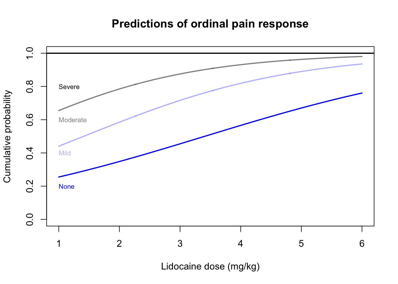
Let’s apply this generalized ordinal logistic regression model to the simulated pain data. For now we will not include hair color, but simply model the ordinal response of pain as a function of the continuous predictor dose.
As expected, higher doses of lidocaine are associated with higher probabilities of no pain and lower probabilities of mild, moderate,or especially severe pain.
The non-linear curves in the graph show how different doses create different probabilities of each pain response. However, we are still using a GLM framework, which means that on the scale of the link function we are still creating linear models. Let’s examine this same model on the scale of the log-odds of each cumulative probability:
Code
plot(x=c(1,6),y=c(-2,4),type='n',main='Predictions of ordinal pain response',ylab='Cumulative log-odds',xlab='Lidocaine dose (mg/kg)')lines(x=xseq$dose,y=predictvglm(pain.olr,newdata=xseq,type='link')[,1],col=pocolors[1],lwd=2)lines(x=xseq$dose,y=predictvglm(pain.olr,newdata=xseq,type='link')[,2],col=pocolors[2],lwd=2)lines(x=xseq$dose,y=predictvglm(pain.olr,newdata=xseq,type='link')[,3],col=pocolors[3],lwd=2)text(x=1,c(-1.5,-0.5,0.5,1.5),levels(pain_cat),adj=0,col=pocolors,cex=0.7)
Here we can start to see a few drawbacks to the generalized ordinal regression. Consider:
This general model is “expensive”, in terms of its model parameters. Every level of our ordinalresponse receives its own regression: each predictor’s effect on cumulative probability is different at each level of \(Y\). If we had five predictors and eight levels to \(Y\), we would be fitting 42 parameters (5 slopes plus an intercept = 6 betas for each of 8 - 1 = 7 levels).
We have to hope the regression slopes remain “well-behaved” or else they may give nonsense predictions. Since the slopes of the linear predictors are not equal to each other, they are not parallel and may well intersect each other. This in turn would lead to impossibilities such as \(P(Y = 1) \gt P(Y \le 2)\). In the graph above, the boundaries are sensible for any realistic dose amount, but this was simply good luck on our part, not an innate model property.
The model doesn’t really set our imagination on fire… it has some subtle differences from the multinomial model, but it seems like a lot of cumbersome math to end up in a very similar place!
Well, I have good news: by adding one bold assumption to this generalized model, we can address all these difficulties!
The proportional-odds ordinal logistic regression (POLR)
What we need now is a “less is more” approach. From the figure above, you may notice that the linear predictors which separate the various cumulative log-odds are almost parallel. What if we assumed they were parallel? In that case, we could simplify our model:
Here we use only one set of slopes for every level of \(Y\), which creates parallel linear predictors on the link scale. The only parameter which varies between levels is the intercept. In order to split out the level-varying intercepts from the fixed vector of slopes \(\hat{\boldsymbol{\beta}}\), we relabel each intercept as \(\hat{\theta}_j\) (theta). In other words, \(\theta\) is the new \(\beta_0\).5
The figure above shows this model in action, modeling the same pain data as before. As each level has a parallel dosage slope, there are only four parameters to estimate:
This reduced model is often quite nearly as good a fit as the generalized model described above. Furthermore, when we choose the logit link, we gain a nice mathematical result called the proportional odds assumption. For any response level \(j\), and any two values of the predictor \(x_0\) and \(x_1\), notice that:
As a corollary, notice that if any single predictor \(X\) is coded as a 1/0 indicator variable, we can further simplify:
\[\frac{\textrm{odds}(Y \le j \,|\, X = 1)}{\textrm{odds}(Y \le j \,|\, X = 0)} = \frac{e^{\theta_j - \beta_X}}{e^{\theta_j}} = e^{-\beta}\]
The beauty and the surprise of these results is that they did not depend at all on the response level \(j\). Instead, these odds ratios are true across every level of \(Y\). A one-unit change in a predictor will have nonlinear effects on the fitted probabilities, but in general the cumulative odds for every level will shift proportionally by the same factor of \(e^{\beta}\).
This property emerges from a combination of (i) using the logit link, and (ii) restricting the model to use only a single set of slopes. We may keep the constraint assumption (ii) while changing the link function (i), in which case we cannot call it the “proportional odds model” because we will no longer be modeling odds.6
Latent variables interpretation
The proportional odds model described above is useful on its own, without any theoretical justification. Data science will always have a home for models that work — i.e. that effectively model real data — whether or not they are known to be “true” or “right” for the data.7
However, we can describe a latent variable interpretation which would motivate these models and even help us to understand which link function to choose.8
Imagine a latent variable \(Z\) which contains rich information about how the predictors affect the ordinal response \(Y\). Define,
Where \(\mathbf{X}\boldsymbol{\beta}\) is the information contained in the predictors and \(\varepsilon\) is a random error term with cumulative distribution function \(F_\varepsilon\). This form should be very familiar to us, since if \(\varepsilon\) has the Normal distribution, then we have “re-invented” linear regression!
Now imagine that we cannot observe \(Z\) directly, but instead, based on its hidden values, we observe the \(j\) different ordinal levels of \(Y\):
So \(Z\) is the continuous hidden variable, and \(Y\) is the observed, flattened “stair-step” which becomes our ordinal response. The values \(\theta_j\) are the cutoff points that determine how \(Z\) maps to \(Y\). Assuming all this to be true, we can write:
(Notice how the latent variable \(Z = \mathbf{X}\boldsymbol{\beta} + \varepsilon\) creates the unusual negative sign in our ordinal linear predictor.) Comparing this with our first description of proportional odds logistic regression, we see that:
If the latent error term \(\varepsilon\) has the logistic distribution, then \(F^{-1}_\varepsilon\) is the logit link and we have recreated the proportional odds model.
If the latent error term \(\varepsilon\) has the Normal distribution, then \(F^{-1}_\varepsilon\) is the probit link which is also used in ordinal regression.
If the latent error term \(\varepsilon\) has the extreme value distribution, then \(F^{-1}_\varepsilon\) is the complementary log-log link.9
We can even visualize the latent variable \(Z\) in such a way as to show the ordinal intercepts \(\theta_j\) serving as cutoff points for the ordinal levels of \(Y\). In the graph below, we choose the logistic distribution for \(F_\varepsilon\), though it looks very similar to the Normal distribution.
Code
plot(x=c(2,7),y=c(-7,3),type='n',main='Latent variable distributions for five doses',xlab='Lidocaine dose (mg/kg)',ylab='Latent variable Z')cutoffs <-rbind(qlogis(0.02,(2:6)*pain.polr$coefficients),matrix(c(pain.polr$zeta),nrow=3,ncol=5),qlogis(0.98,(2:6)*pain.polr$coefficients))pocolors <-c('#0000ff','#0000ff50','#00000080','#000000')abline(h=pain.polr$zeta,col=pocolors[1:3])for (x in1:5){for (y in1:4){ poseq <-seq(cutoffs[y,x],cutoffs[y+1,x],length.out=100)lines(x=rep(x+1,100),y=poseq,lwd=2,col=pocolors[y])lines(x=x+1+2*dlogis(poseq,(x+1)*pain.polr$coefficients),y=poseq,lwd=2,col=pocolors[y])if (x==1) text(x=7,y=y-3,levels(pain_cat)[y],adj=1,col=pocolors[y],cex=0.7)}}mtext(text=expression(theta[1]),side=4,at=c(7,pain.polr$zeta[1]),las=2,line=0.5)mtext(text=expression(theta[2]),side=4,at=c(7,pain.polr$zeta[2]),las=2,line=0.5)mtext(text=expression(theta[3]),side=4,at=c(7,pain.polr$zeta[3]),las=2,line=0.5)
Latent variables interpretation of proportional odds logistic regression
Choosing the right link function for your data
Just like binomial regression, ordinal regression can be modeled using a variety of links, which have been hinted at in the descriptions above. The most common link choice is probably logit, but probit and complementary log-log models are also common, perhaps even moreso than in modeling binomial data. How should we choose which link function to use?
The advice given in Building new GLMs still holds: sometimes we pick a link because we believe in the process, and sometimes we pick a link simply because we notice that the model well explains the data. Familiar tools such as AIC and RMSE can help us to judge the model fit and predictive power.
But what about the process? How do we enter a problem with an a priori (though testable) assumption of which link to use? I suggest a few considerations below.
Use a logit link when:
The proportional odds interpretation is extremely helpful to your audience, as a rubric for effect size or decision-making. Examples might include medical specialties (say, surgery or oncology) where odds ratios are commonly used to discuss and choose between different treatment plans.
You are extending an earlier binomial logistic regression model to include a third choice.
You don’t know any better! It’s a fine default link.
Use a probit link when:
You believe the data are generated by a latent variable with Normally-distributed errors, which often happens as the result of summing many independent contributing factors. Examples might include dose-response models for the effects of poison or radiation: each person or specimen has a ‘natural resistance’ which might be Normally distributed as the result of many different genetic and environmental factors.
Your audience is more comfortable with z-scores than with log-odds (as is often true in economic or social scientific research fields).
You don’t need to use a proportional-odds or proportional-hazards interpretation, e.g. if all you need are a good set of predictions.
Use a complementary log-log link or negative log-log link when:
You believe the underlying latent variable has a strongly asymmetric distribution. Examples might include brand recognition as backed by the latent variable of market penetration (it’s very common to have \(<20\%\) market share but very uncommon to have \(>80\%\) market share.)
You believe the underlying latent variable specifically comes from an extreme value distribution. For example, imagine rating the taste of many bottles of old wine which should be kept at an ideal temperature and humidity to prolong their life. Each bottle could spend 50 years in ideal conditions, but one bad day (perhaps a power outage) could have a serious effect on their flavor. In this scenario, the ordinal rating of wine quality is linked to the latent variable which measures the most extreme conditions which the bottle ever faced.
The proportional hazard interpretation is helpful to your audience, i.e. the Cox proportional hazards model. These models are commonly used with continuous-time survival models, for instance in predicting the number or severity of machine failures on a factory floor.
Although this is true of many different countries, the specific parties or positions which mark the extremes of one country’s political spectrum might fall in the middle for a different country!↩︎
For example, we could model military officer ranks as a categorical variable with 10 levels, but we would not be using the knowledge that an O-4 major is meaingfully “between” an O-3 captain and an O-5 lieutenant colonel.↩︎
Although these doses are realistic, they should not be confused with real observations or used for medical decisionmaking!↩︎
Usually we add the slopes and \(X\)s to the intercept term, but you see here that we subtract\(\mathbf{X} \hat{\boldsymbol{\beta}}\) from \(\hat{\theta}_j\). We can choose either sign arbitrarily and without changing the math of the model, and we choose this expression so as to neatly phrase the latent variable interpretation below.↩︎
Though other properties may emerge… if we use the complementary log-log link function, we reach a very similar result referred to as the “proportional hazard model”.↩︎
Note: This section owes a particular debt not only to McCullagh and Nelder’s Generalized Linear Models 2nd edition, but also to some notes of Professor McCullagh available at https://www.stat.uchicago.edu/~pmcc/reports/prop_odds.pdf↩︎
Or the negative log-log link, if the extreme values are minima and not maxima.↩︎