We have learned how to identify the best guess for an unknown parameter from the data. We have also learned how to check if a specific alternative is a reasonable guess, or if the data make it too unlikely to be true. Now we shall learn how to find the range of all reasonable guesses for an unknown parameter. This range is called a confidence interval, because the size of the range depends on how confident we are that it will contain the true parameter:
If we pick wide ranges, we can be confident that they will actually include the true parameter, but the range might be so wide that we don’t gain useful or actionable information.
If we pick narrow ranges, we seem much more precise in our estimates, but we run a greater risk of being wrong about where the true parameter is located.
You are the one who decides how confident to be. Combining your own risk tolerance with the precise nature of the problem at hand, you choose a confidence level, usually a number close to 100%. Then you find the upper and lower bounds for your interval.
Definition… well, more or less
I wish I could now show you how to construct a confidence interval. Many other textbooks do, at this point. But the truth is, confidence intervals are very poorly defined(?!) and statisticians do not agree on how best to build them(!!). For the moment, I will leave you with an unsatisfying half-answer: what a confidence interval should do.
Note
Let \(\theta \in \mathcal{S}\) be a parameter from a random variable \(X\) and let \(\boldsymbol{x}\) be an as-yet unobserved sample from \(X\). Suppose that \(a(\boldsymbol{x})\) and \(b(\boldsymbol{x})\) are also random variables that are functions of the sample (that is, their values will vary sample to sample). If,
for all samples and all parameter values $, then \([a(\boldsymbol{x}),b(\boldsymbol{x})]\) is a \(1 - \alpha\)confidence interval for the true value of the parameter \(\theta\).
Example 1: Exact binomial confidence interval
I will show you one example of an exact confidence interval below, and in the next chapter I will show you a method for constructing approximate confidence intervals which are much easier to calculate and which are very accurate for large sample sizes.
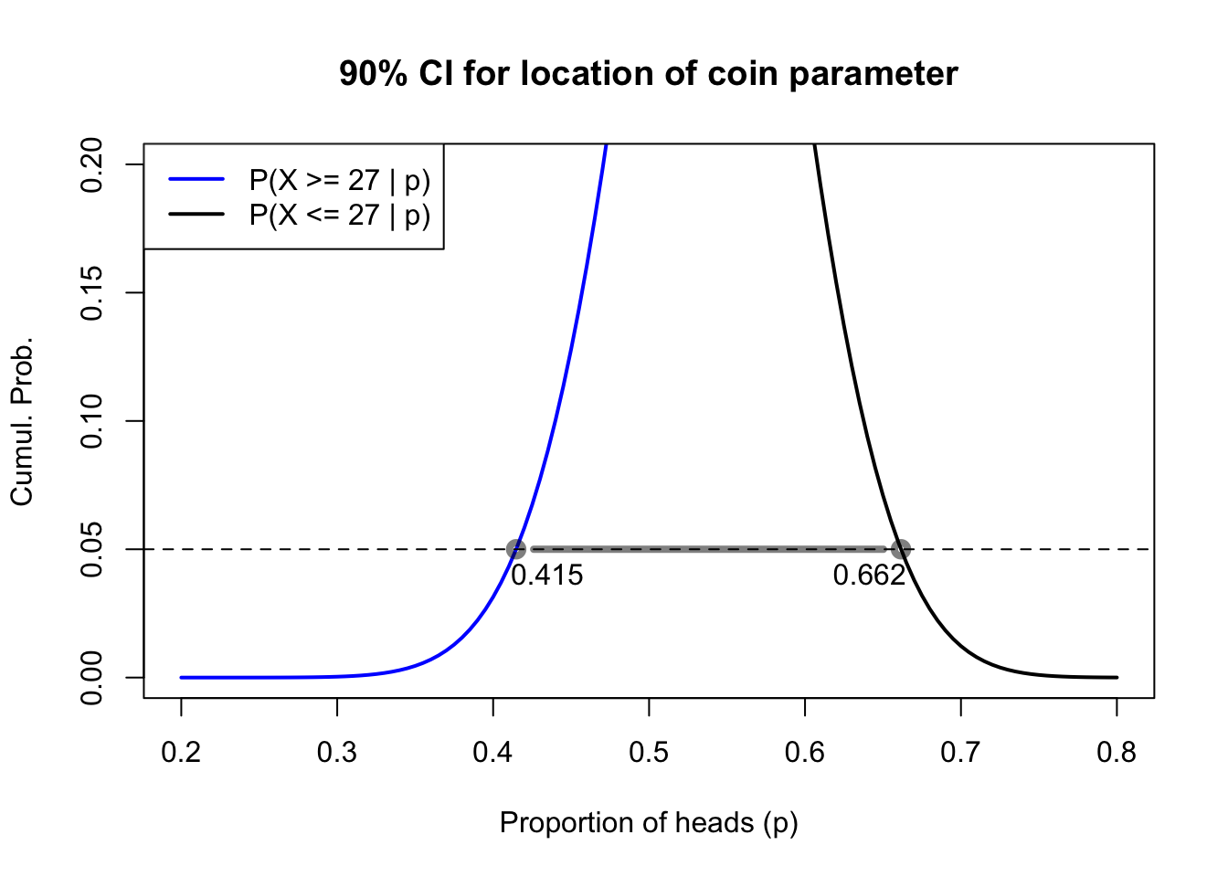
Let’s return to the coin data: 27 heads from 50 trials. We’ve already shown that a fair 50-50 coin could reasonably have produced this sample. We’ve also shown that an unfair 40-60 coin would not likely have produced this sample. Using a computer’s help and the CDF of the binomial distribution, I can find the exact lower and upper bounds \(p^*_{l,0.05}\) and \(p^*_{u,0.05}\) such that:
If \(p\) were any lower than \(p^*_{l,0.05}\), then observing so many heads (27 or more) would happen less than 5% of the time
If \(p\) were any higher than \(p^*_{u,0.05}\), then observing so few heads (27 or fewer) would happen less than 5% of the time
When I use this method to build a confidence interval, I know that 10% of the time my data is going to “trick” me into constructing an interval which does not include the true parameter. This will happen when — by freak chance — the data contain so many heads (or so many tails) that the true parameter seems like a bad fit to the data. But 90% of the time the interval I create will contain the true parameter. Even when the data have a few more heads or a few more tails than expected, the true parameter will be among the values that could plausibly create such data. Therefore we say that this method produces an “exact” 90% confidence interval for \(p\).1
Code
#exact 90CI for binomial datapl <-uniroot(function(z){pbinom(26,50,z)-0.95},interval=c(0.3,0.7))$rootpu <-uniroot(function(z){pbinom(27,50,z)-0.05},interval=c(0.3,0.7))$rootplot(seq(0.2,0.8,0.005),1-pbinom(26,50,seq(0.2,0.8,0.005)),type='l',col='#0000ff',lwd=2,ylim=c(0,0.2),xlab='Proportion of heads (p)',ylab='Cumul. Prob.',main='90% CI for location of coin parameter')lines(seq(0.2,0.8,0.005),pbinom(27,50,seq(0.2,0.8,0.005)),type='l',col='#000000',lwd=2)abline(h=0.05,lty=2)lines(x=c(pl,pu),y=c(0.05,0.05),type='b',col='#00000080',lwd=4)legend(x='topleft',legend=c('P(X >= 27 | p)','P(X <= 27 | p)'),col=c('#0000ff','#000000'),lwd=2)text(x=c(pl+0.02,pu-0.02),y=c(0.05,0.05),pos=1,labels=round(c(pl,pu),3))
Figure 4.1: Construction of an exact binomial confidence interval
Exact normal confidence intervals (two-sided)
Discrete and asymmetric distributions both pose particular challenges for defining an exact confidence interval. The normal distribution provides a somewhat more convenient case. Let us consider the most general case first, so that we can try to find a method which will work for all normally-distributed samples.
Assume that we have a sample \(\boldsymbol{x} = \{x_1, \ldots, x_n\}\) which observes a normally-distributed random variable \(X\) with unknown mean \(\mu_X\) and known variance \(\sigma^2_X\).2 How might we compute a \((1-\alpha)\) confidence interval for the mean of \(X\)?3
Lower bound
The lower bound would be a potential true mean \(x^*_{l,\alpha/2}\) for which these observations would be unusually large; in fact, if \(\mu = x^*_{l,\alpha/2}\) then samples as large as \(\boldsymbol{x}\) would be seen with probability \(\alpha/2\)].4
Since we our sample has many observations, what precisely does it mean to be “unusually large”? Recall that the average of independent and identically-distributed normal variates is also normally distributed:
Note
If \(X_1, \ldots, X_n\) are each normally distributed random variables with mean \(\mu_X\) and variance \(\sigma_X^2\), then:
From this handy result, we can define a more “extreme” or “unusual” sample as one with a sample average further from the mean.
Now we can back out the critical value of \(\mu^*_{l,0.05}\). Let \(\bar{X}\) be our normally distributed sample mean, centered on our unknown \(x^*_{l,\alpha/2}\) and with standard deviation \(\sigma_X/\sqrt{n}\). Notice that we can standardize this normal variable without losing any information: if we define \(Z = (X - x^*_{l,\alpha/2})/(\sigma_X/\sqrt{n})\), then \(Z \sim \mathrm{Normal}(0,1)\).
With complete symmetry, we define the upper bound of our interval as the hypothetical mean for which our data seem unusually and improbably small; in fact, that such “small” samples would only occur with probability \(\alpha/2\). Using the same methods shown above, we conclude,
With the general solution now in hand, let’s try computing a specific example.
Example 2: Pulsar distances
Imagine that astronomers discover a new pulsar in deep space.5 To use the new pulsar’s data effectively, we need to know how far away it is, but our measurements of deep-space distance are very imprecise. We believe each measurement is normally distributed around the true distance with standard deviation of 7.5 light years. Astronomers take ten measurements:
From which we may conclude that the pulsar is truly between 408.9 and 416.7 light years away. Of course, we could be wrong! We have no guarantee of this conclusion. But the method we used is right 95% of the time, at least when we are correct in our assumptions about the data being independent and identically normally distributed with a known standard deviation.
Misconceptions about confidence intervals
We will learn more about confidence intervals soon. But while we are discussing theory, I want to emphasize a few common misunderstandings about their concept and purpose. For the sake of argument, let’s say that you have a calculated a 95% confidence interval.
FALSE: “95% of the values of the distribution are inside the interval”
We are not trying to define or bound the overall distribution. We are only talking about a property of the distribution: a parameter like its mean, or its endpoints, or the slope in a regression.
FALSE: “The true parameter has a distribution described by our interval.”
The true parameter isn’t randomly distributed, or distributed at all: it’s just unknown. If our data only misleads us a little, it will be inside our interval. If our data misleads us a lot, the true parameter will be outside the interval. We don’t know how much our data is misleading us.
FALSE: “There’s a 95% chance that this interval contains the true parameter.”
Again, we are not talking about a probabilistic event. Once the interval has been calculated, there are no varying components. Our endpoints are fixed. The truth of where the parameter is was fixed before we woke up this morning, possibly before we were born. We are either right or wrong, and we don’t know which.
TRUE: “The process which created this interval successfully covers the true parameter in 95% of its applications.”
We don’t know if this specific interval is right or wrong, but we know the process usually results in success.
Visualizer: Confidence interval success and failure
The visualizer below allows you to construct many confidence intervals for normally-distributed data with variance 1. The true data is standard normal, that is, \(\mathrm{Normal}(0,1)\). However, individual samples may mislead us — if the sample average is much higher or lower than zero, we may not believe that 0 could be the true mean. Intervals containing the true mean of zero are colored blue, intervals which wrongly exclude the true mean will be colored red.
#| '!! shinylive warning !!': |
#|   shinylive does not work in self-contained HTML documents.
#|   Please set `embed-resources: false` in your metadata.
#| standalone: true
#| viewerHeight: 500

library(shiny)
library(bslib)

ui <- page_fluid(
  tags$head(tags$style(HTML("body {overflow-x: hidden;}"))),
  title = "Confidence interval builder for normal data",
  fluidRow(column(width=5,sliderInput("nsamp", "N (sample size)", min=5, max=200, value=25)),
           column(width=5,sliderInput("conf", "Confidence", min=80, max=99, post='%', value=95)),
           column(width=2,actionButton("go","Generate!"))),
  fluidRow(column(width=12,plotOutput("distPlot1"))))

server <- function(input, output) {
  output$distPlot1 <- renderPlot({
    input$go
    x <- isolate(rnorm(input$nsamp))
    p <- isolate(1-(100-input$conf)/200)
    xlo <- mean(x) - qnorm(p)/sqrt(length(x))
    xhi <- mean(x) + qnorm(p)/sqrt(length(x))
    good <- (xlo < 0) & (xhi > 0)
    plot(x=x,y=rep(-1,length(x)),pch=4,cex=2,xlim=c(-3.5,3.5),ylim=c(-2,2),axes=FALSE,ylab=NA,xlab='Values of X')
    axis(1,-3:3,-3:3,pos=0)
    lines(x=c(xlo,xhi),y=c(1,1),lwd=5,type='b',col=c('red','blue')[1*good+1])
    text(x=c(xlo,xhi),y=c(1,1),pos=c(2,4),labels=round(c(xlo,xhi),2))
    abline(v=mean(x),lty=2)})
}

shinyApp(ui = ui, server = server)
This particular method is known as the Clopper-Pearson interval. But as if to illustrate the confusion on this topic, it is neither the only “exact” calculation nor the one with the best performance!↩︎
In practice it’s incredibly rare to know the variance without knowing the mean. This will be addressed in The Student’s t distribution.↩︎
E.g. if we wanted a 95% confidence interval, then we would set \(\alpha = 0.05\).↩︎
E.g. if we are computing a 95% confidence interval, samples so large would only be seen 2.5% of the time.↩︎
Pulsars are star-like objects which emit energy at extremely regular intervals, making them very valuable for mapping the universe, terrestrial timekeeping, and interstellar navigation.↩︎