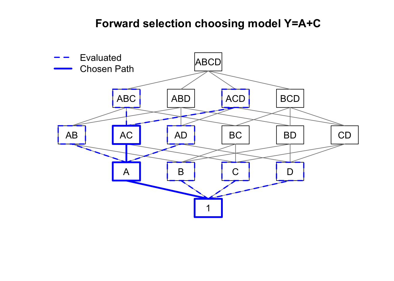
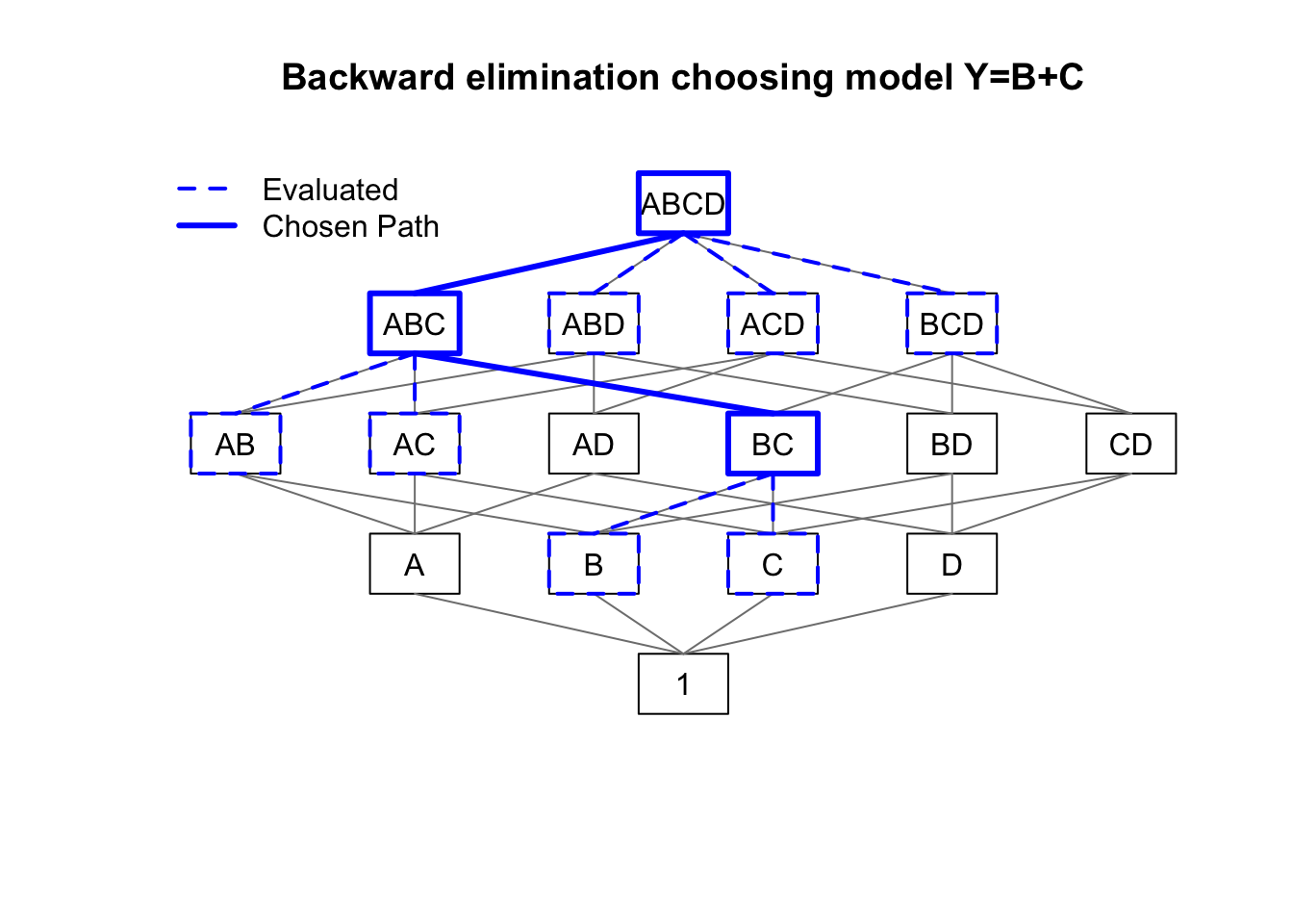
plot(runif(1),runif(1),type='n',xlim=c(-11,11),ylim=c(1,19),
     axes=FALSE,xlab='',ylab='',
     main='Backward elimination choosing model Y=B+C')
rect(xleft=c(-1,-7,-3,1,5,-11,-7,-3,1,5,9,-7,-3,1,5,-1),
     ybottom=c(1,5,5,5,5,9,9,9,9,9,9,13,13,13,13,17),
     xright=c(1,-5,-1,3,7,-9,-5,-1,3,7,11,-5,-1,3,7,1),
     ytop=c(3,7,7,7,7,11,11,11,11,11,11,15,15,15,15,19))
text(x=c(0,-6,-2,2,6,-10,-6,-2,2,6,10,-6,-2,2,6,0),
     y=c(2,6,6,6,6,10,10,10,10,10,10,14,14,14,14,18),
     labels=c('1','A','B','C','D','AB','AC','AD','BC',
              'BD','CD','ABC','ABD','ACD','BCD','ABCD'))
segments(x0=c(0,0,0,0,-6,-6,-6,-2,-2,-2,2,2,2,6,6,6,
              -10,-10,-6,-6,-2,-2,2,2,6,6,10,10,-6,-2,2,6),
         y0=c(rep(3,4),rep(7,12),rep(11,12),rep(15,4)),
         x1=c(-6,-2,2,6,-10,-6,-2,-10,2,6,-6,2,10,-2,6,10,
              -6,-2,-6,2,-2,2,-6,6,-2,6,2,6,0,0,0,0),
         y1=c(rep(5,4),rep(9,12),rep(13,12),rep(17,4)),col='grey50')
segments(x0=c(rep(0,4),rep(-6,3),rep(2,2)),
         y0=c(rep(17,4),rep(13,3),rep(9,2)),
         x1=c(-6,-2,2,6,-10,-6,2,-2,2),
         y1=c(rep(15,4),rep(11,3),rep(7,2)),
         col='#0000ff',lwd=c(3,2,2,2,2,2,3,2,2),lty=c(1,2,2,2,2,2,1,2,2))
rect(xleft=c(-1,-7,-3,1,5,-11,-7,1,-3,1),
     ybottom=c(17,13,13,13,13,9,9,9,5,5),
     xright=c(1,-5,-1,3,7,-9,-5,3,-1,3),
     ytop=c(19,15,15,15,15,11,11,11,7,7),
     border='#0000ff',lwd=c(3,3,2,2,2,2,2,3,2,2),lty=c(1,1,2,2,2,2,2,1,2,2))
legend(x='topleft',bty='n',lty=c(2,1),lwd=c(2,3),
       legend=c('Evaluated','Chosen Path'),col='#0000ff')