In Univariate likelihood, we learned to maximize likelihood functions using arithmetic and calculus. However, sometimes the likelihood function does not allow a closed-form solution, and of course modern computers do not solve problems with pencil and paper. How then would we find the maximum of an unsolvable likelihood equation?
The short answer is that we can use any of several algorithmic optimization methods. These methods were not developed specifically for statistical use, but they work quite well for our purposes, and we can easily express them in machine-readable code. One example of these optimization algorithms is the Newton-Raphson method, which has been used for hundreds of years.1
Definition
The Newton-Raphson method specifically finds the root of an equation, i.e. the value of \(x\) for which the function’s value \(f(x)\) is zero. We can use this to find where the first derivative of a log-likelihood function is zero, which in turn will (usually) be the maximum of the original likelihood function:2
Note
Let \(f\) be a continuous and differentiable function with derivative \(f'\) and at least one root, i.e. there exists some \(x^*\) such that \(f(x^*) = 0\). The root \(x^*\) can sometimes be approximated, depending on the nature of the function \(f\) and the choice of an initial guess \(x_0\), by successively iterating the following series:
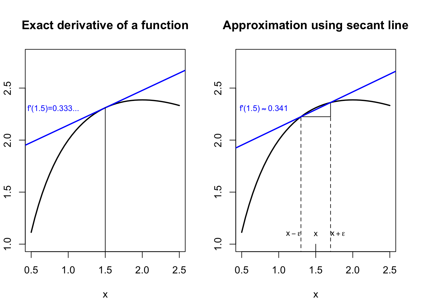
When we have a perfect algebraic expression for the derivative \(f^{'}\), then we should by all means use it. But if we don’t have a closed-form solution, or if we are using computers to speed our work, we may approximate the derivative with a local linearization. If you were taught calculus through the concept of infinitesimals, this formula may be familiar. Rather than compute the slope of an exact tangent line, we can compute the slope of a secant line between two very nearby points, as shown in the equation and figure below:
#secant approximation to the derivativepar(mfrow=c(1,2),mar=c(4,2,4,2)+0.1)sec.x <-seq(0.5,2.5,0.05)fsec <-function(x) 2*log(x)-x+3plot(sec.x,fsec(sec.x),type='l',lwd=2,ylim=c(1,2.8),main='Exact derivative of a function',xlab='x',ylab='f(x)')abline(fsec(1.5)-0.5,1/3,col='#0000ff',lwd=2)lines(x=c(1.5,1.5),y=c(0,fsec(1.5)))text(0.8,2.3,"f'(1.5)=0.333...",col='#0000ff',cex=0.8)plot(sec.x,fsec(sec.x),type='l',lwd=2,ylim=c(1,2.8),main='Approximation using secant line',xlab='x',ylab='f(x)')lines(x=c(1.3,1.3),y=c(0,fsec(1.3)),lty=2)lines(x=c(1.7,1.7),y=c(0,fsec(1.3)),lty=2)lines(x=c(1.3,1.7),y=c(fsec(1.3),fsec(1.3)))lines(x=c(1.7,1.7),y=c(fsec(1.3),fsec(1.7)))lines(x=c(1.5,1.5),y=c(0,1))sec.b <- (fsec(1.7)-fsec(1.3))/0.4abline(fsec(1.3)-1.3*sec.b,sec.b,1/3,col='#0000ff',lwd=2)text(0.8,2.3,expression("f'(1.5)"%~~%0.341),col='#0000ff',cex=0.8)text(1.5,1.1,expression(x),cex=0.8)text(1.2,1.1,expression(x-epsilon),cex=0.8)text(1.8,1.1,expression(x+epsilon),cex=0.8)
Figure 7.1: Approximating the derivative with a secant line
Whether we use an exact algebraic solution for the derivative or approximate it with a secant line, we are now ready to use the Newton-Raphson method to produce a MLE:
Compute a log-likelihood function for your parameter
Find the derivative of the log-likelihood function, or estimate it using the secant approximation. You will be trying to find a root for this equation; it is the function \(f\) described in the equations above.
Find the second derivative of the log-likelihood function, or estimate it using the second approximation. You will use this second derivative to iterate the algorithm; it is the function \(f'\) in the equations above.
Choose an initial guess for the root (i.e. the best parameter value.)
Choose a tolerance which will help you know when to stop iterating the algorithm. This tolerance is sometimes expressed as an maximum change in \(x\), or other times as a maximum increment in \(f(x)\) (i.e. the first derivative of the log-likelihood).
Iterate until the new values of \(x\) and \(f(x)\) are within tolerance, or stop the algorithm if your search does not converge upon a root.
Notice that the method I have outlined here only works for functions of a single variable, meaning that it will only work to identify distributions defined by a single parameter. Distributions with multiple parameters are more typically solved through gradient descent, which will be outlined in the next section.
Programming example: coin data
In the code below, I create a general-purpose Newton-Raphson algorithm, which would work in a wide variety of use cases. Then we’ll apply it to a specific dataset.
# helper function to approximate derivativesddx <-function(value, func, delta=1e-6){ (func(value+delta)-func(value-delta))/(2*delta)}# core newton-raphson algorithm, plus some outputnewton <-function(f, x0, tol=1e-6, max.iter=20){ x <- x0 i <-0 results <-data.frame(iter=i,x=x,fx=f(x))while (abs(f(x))>tol & i<max.iter) { i <- i +1 x <- x -f(x)/ddx(x,f) results <-rbind(results,data.frame(iter=i,x=x,fx=f(x)))}return(results)}
1
This implements the secant approximation method shown above
2
The inputs are f (the function whose root we are finding), x0 (an initial guess), a tolerance (we will stop the algorithm when we get this close to a root), and a maximum number of iterations (in case we don’t converge)
3
To show my work, I’m outputting results to a table
4
The algorithm will stop when \(f(x)\) is within tolerance of 0 or when it hits the maximum iteration count without converging
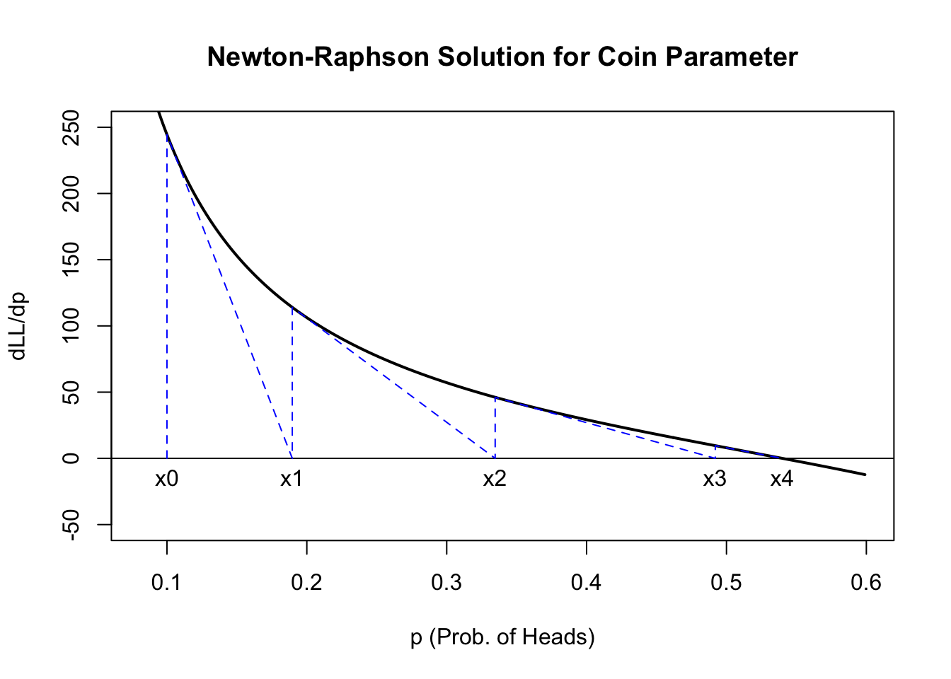
With this new tool, let’s revisit the coin data from Univariate likelihood. I will regenerate the data here, and also code up the derivative of the log-likelihood function:
#coin data generated with true p=0.6set.seed(2061)coins <-sample(0:1,50,TRUE,c(0.4,0.6))# derivative of log-likelihood for coin parametercoin.dll <-function(p) sum(coins)/p-sum(1-coins)/(1-p)
1
Specifying the seed forces the same “random” numbers to occur each time
2
Even though \(p=0.6\), only \(27/50 = 54\%\) of these 50 flips are heads
Finally, I will run the Newton-Raphson algorithm and plot the result. Recall that earlier we found that the true MLE for this coin data was \(\hat{p} = 0.54\):
Notice that the algorithm very quickly finds a root near 0.54 and that the algorithm only stops when the “height” of the function is within the tolerance (here \(1 \times 10^{-6}\)). More complicated likelihood functions and worse initial guesses can lead to non-convergence, but this function was very well-behaved, as you can see below:
Code
plot((81:599)/1000, coin.dll((81:599)/1000),type='l',lwd=2,main="Newton-Raphson Solution for Coin Parameter",xlab='p (Prob. of Heads)',ylab='dLL/dp',ylim=c(-50,250))abline(h=0)lines(x=rep(coin.newt$x,each=2),y=c(rbind(t(rep(0,dim(coin.newt)[1])),t(coin.newt$fx))),col='#0000ff',lty=2)text(x=coin.newt$x[1:5],y=0,labels=paste0('x',coin.newt$iter[1:5]),pos=1)
Figure 7.2: Newton-Raphson approximation of coin MLE
At least four mathematicians could lay claim to this method, and neither Isaac Newton nor Joseph Raphson published first or completed the version we use today. Stigler’s Law of Eponymy strikes again!↩︎
Do be cautious, since the root of a derivative may instead match an inflection point or local minimum of the original function, and the true maximum of a likelihood function may not be a local maximum.↩︎