Code
set.seed(1210)
depth <- sort(floor(c(runif(10,0,40),runif(10,20,60),runif(10,40,80)))/4)
trout <- rpois(30,exp(-1+0.25*depth))
plot(depth,trout,main='Number of lake trout caught each day',
     xlab='Line depth (m)',ylab='Trout caught')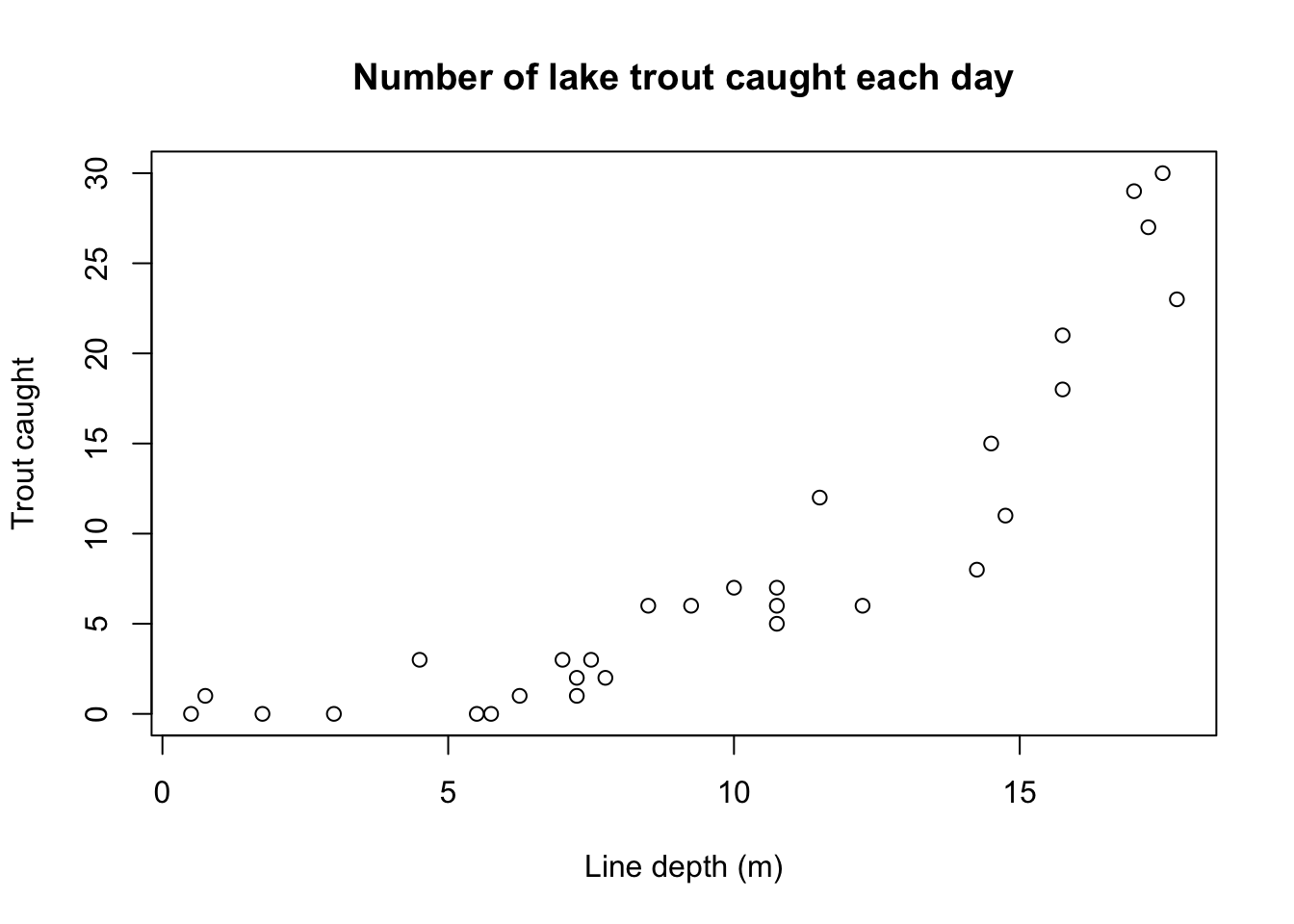
So far, our discussion of GLMs has focused on binary response variables which only take on values of 1 and 0. We began with these examples because they were relatively simple to model and because they expose and amend many of the shortcomings of linear regression. Let’s apply this new model-fitting method to a different type of response variable: count data. Count data assumes a non-negative integer number of outcomes, which typically count a number of events:
The number of calls dropped by a cell tower, as observed over many one hour-long observation windows
The number of spontaneous genetic mutations in a particular stretch of DNA, as observed among many newborn children
The number of Prussian cavalry officers killed by a kick from their own horse, as observed in each of the many years which the Prussian army kept such records
That last example is in fact drawn from real life; the statistician Ladislaus Bortkiewicz studied these same records in 1898 and noticed that the totals closely matched a mathematical formula which had been studied earlier by the mathematicians Abraham de Moivre (in 1711) and Siméon Denis Poisson (in 1837). Bortkiewicz’s work led to the recognition of the Poisson distribution, which serves as an excellent entry point for studying count regressions.
Imagine an experienced freshwater fisher who lives by a large lake and loves to catch lake trout. From prior experience, the fisher knows that trout are often found in deeper waters rather than shallower waters, and now wishes to study this trend with some data. During one summer month, the fisher travels out to different spots on the lake and fishes at different depths each day, for thirty days:
| Depth (m) | 0.50 | 0.75 | 1.75 | 3.00 | 4.50 | 5.50 | 5.75 | 6.25 | 7.00 | 7.25 |
| Caught | 0 | 1 | 0 | 0 | 3 | 0 | 0 | 1 | 3 | 1 |
| Depth (m) | 7.25 | 7.50 | 7.75 | 8.50 | 9.25 | 10.00 | 10.75 | 10.75 | 10.75 | 11.50 |
| Caught | 2 | 3 | 2 | 6 | 6 | 7 | 6 | 7 | 5 | 12 |
| Depth (m) | 12.25 | 14.25 | 14.50 | 14.75 | 15.75 | 15.75 | 17.00 | 17.25 | 17.50 | 17.75 |
| Caught | 6 | 8 | 15 | 11 | 18 | 21 | 29 | 27 | 30 | 23 |
Plotting these records, the fisher notices a direct but nonlinear trend:
set.seed(1210)
depth <- sort(floor(c(runif(10,0,40),runif(10,20,60),runif(10,40,80)))/4)
trout <- rpois(30,exp(-1+0.25*depth))
plot(depth,trout,main='Number of lake trout caught each day',
xlab='Line depth (m)',ylab='Trout caught')
How should we model this data? We face some difficult constraints: nonlinearity, heteroskedasticity (note how range of count values opens up as depth increases), and non-normality (counts can only be integer-valued and non-negative, which creates extremely non-normal error distributions, especially for shallow depths.)
Let’s assume that the counts come from a Poisson distribution. We can feel comfortable with this starting point because, at least on the surface, fishing resembles a Poisson process. There are a large (essentially infinite) number of possible events (fish in the lake), and a low probability of catching any specific one of them. You can’t catch two fish at once, and the number of fish caught might be roughly proportional to the time spent fishing. Fish are probably not caught independently from each other, but Poisson still seems like a fine starting place.
As detailed in the appendices, the Poisson distribution PMF takes the form:
\[P(Y=y) = \lambda^y e^{-λ} / y! \]
Where \(\lambda\), the rate or intensity of the Poisson process, is both the mean and the variance of the distribution. Since \(\mu = \lambda\), if we use the Poisson for the distributional assumption of a GLM model, then we must choose some link function \(g\) such that \(g(\mu) = \mathbf{X}\boldsymbol{\beta}\). Then for each observation \(i\) we would have \(\lambda_i = \mu_i = g^{-1}(\boldsymbol{x}_i\boldsymbol{\beta})\), and our GLM would have the form,
\[P(Y_i=y_i) = \lambda_i^{y_i} e^{-\lambda_i} ⁄ y_i!\]
Put another way, in a Poisson regression, each observation \(y_i\) is drawn from a Poisson distribution with rate \(\lambda_i\), which is also the mean and the variance, and this rate is a (possibly nonlinear) function of the linear predictor \(\boldsymbol{x}_i\boldsymbol{\beta}\).
The canonical link for the Poisson GLM is the log link, which claims that \(\log \mu = \log \lambda = \mathbf{X}\boldsymbol{\beta}\) and therefore \(\mu = \lambda = e^{\mathbf{X}\boldsymbol{\beta}}\). One of the advantages of this log link is that no matter how large, small, or negative our linear predictor \(\mathbf{X}\boldsymbol{\beta}\), the mean function \(e^{\mathbf{X}\boldsymbol{\beta}}\) will always be positive, which is a requirement for \(\lambda\) in the Poisson distribution.1
Nothing requires your predictors and your Poisson process rates to relate to each other in this way. Just as with the binary GLMs in previous sections, some problems will be a solid theoretical fit for this link, other problems will happen to be modeled well by this link, and still other problems will be poorly modeled by this link.
Let’s fit this model to the trout fishing data above and see where it leads us:
trout.log <- glm(trout~depth,family=poisson)
summary(trout.log)| Parameter | Estimate | p-value |
|---|---|---|
| \(\beta_0\) (Intercept) | -0.808 | <0.0001 |
| \(\beta_1\) (Line depth) | 0.237 | <0.0001 |
| \(\;\) | ||
| Null deviance | 283.426 | (29 df) |
| Model deviance | 29.039 | (28 df) |
By comparing the null deviance to the model deviance, we know this model fits the trout data significantly better than a null model in which one fixed Poisson rate \(\lambda\) generated all 30 fishing counts.2 (Consider that the sample mean was 8.43 trout while the sample variance was 85.84… a bad look for a distribution where the two are assumed equal.)
By examining the model deviance by itself, we know this model does not fit the data significantly worse than the saturated model, which assigns every observation its own individual Poisson rate (i.e. its own mean).3 In other words, we could terribly overfit the model by saying that the expectation for each day’s fishing trip was exactly how many fish were actually caught… and yet we have almost the same degree of fit with just a single slope on fishing depth.
What about the coefficients? What does each parameter estimate \(\hat{\beta}_k\) represent?
\(\hat{\beta}_0\), the intercept, is the predicted log of the Poisson rates whenever all the predictors are set to 0. In this situation, \(e^{\hat{\beta}_0}\) is the predicted mean and the predicted Poisson rate. For our fishing data, that suggests that fishing at a depth of 0 m (letting your bait float on top of the water) yields an expected daily catch of only \(e^{-0.808} \approx 0.446\) trout. Using the Poisson distribution we can further calculate a 64% chance of catching no trout, a 29% chance of one trout, a 6% chance of two trout, and only a 1% chance of three or more trout. The intercept does not always describe an interesting or realistic scenario, but here it did.
\(\hat{\beta}_1\), the slope on the first predictor describes a nonlinear trend, similar to the coefficients in logistic or probit regression. Consider incrementing \(X_1\) by one: \(x_{1,\textrm{new}} = x_{1,\textrm{old}} + 1\). Then we would have:
\[\begin{aligned} \hat{y}_\textrm{new} = \hat{\mu}_\textrm{new} &= e^{\hat{\beta}_0 + \hat{\beta}_1 x_{1,\textrm{new}}} = e^{\hat{\beta}_0 + \hat{\beta}_1 (x_{1,\textrm{old}} + 1)} \\ &= e^{\hat{\beta}_0 + \hat{\beta}_1 x_{1,\textrm{old}} + \hat{\beta}_1} = e^{\hat{\beta}_0 + \hat{\beta}_1 x_{1,\textrm{old}}} \cdot e^{\hat{\beta}_1} \\ &= \hat{\mu}_\textrm{old} \cdot e^{\hat{\beta}_1} \end{aligned}\]
So, a one-unit change in \(X_1\) multiplies the mean (and the variance, and the Poisson rate) by a factor of \(e^{\hat{\beta}_1}\). If \(\hat{\beta}_1\) is positive then increasing \(X_1\) will tend to increase \(Y\). If \(\hat{\beta}_1\) is negative then increasing \(X_1\) will tend to decrease \(Y\). For our fishing data, we see that \(e^{\hat{\beta}_1} \approx 1.267\), meaning that for each meter deeper we fish, the expected daily catch increases by 26.7%.
Any further coefficients \(\hat{\beta}_j\) paired with predictors \(X_j\) behave just as \(\hat{\beta}_1\) did above.
With these betas we can also directly estimate the probabilities of individual count outcomes. Recall that for a linear regression, the predicted mean \(\hat{\mu}_i\) was also our best guess of the actual value of an observation \(\hat{y}_i\) and that \(\hat{\mu}_i = \hat{y}_i = \boldsymbol{x}_i \hat{\boldsymbol{\beta}}\). A Poisson regression differs because the values of \(Y\) are integers: in most situations, \(y_i\) could never be \(\mu_i\). Still, since we know that \(\hat{\mu}_i = \hat{\lambda}_i\), we can use the Poisson PMF to compute the probability that \(\hat{y}_i=0\), that \(\hat{y}_i=1\), that \(\hat{y}_i=2\), and so on.
plot(depth,trout,main='Predictions of Poisson log link GLM',
     xlab='Line depth (m)',ylab='Trout caught',pch=19)
lines(seq(0,19,0.1),exp(predict(trout.log,newdata=list(depth=seq(0,19,0.1)))),
      lty=2,col='grey50',lwd=2)
lines(seq(0,19,0.1),qpois(0.1,exp(predict(trout.log,newdata=list(depth=seq(0,19,0.1))))),
      col='#0000ff',type='s')
lines(seq(0,19,0.1),qpois(0.9,exp(predict(trout.log,newdata=list(depth=seq(0,19,0.1))))),
      col='#0000ff',type='s')
legend(x='topleft',col=c('black','grey50','#0000ff'),lty=c(NA,2,1),lwd=c(NA,2,1),pch=c(19,NA,NA),
       legend=c('Observations','Estimated mean','Estimated 80% of outcomes'))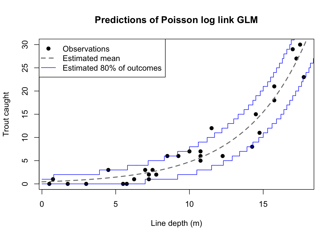
The figure above re-plots the trout catches alongside a curved line representing the fitted mean trout catch (also the fitted Poisson intensity) at each depth. The figure also shows bounds corresponding to the 10th and 90th percentiles from the Poisson distribution with these same fitted intensities. This window isn’t a confidence interval. It simply assumes that the fitted means are exactly correct (they won’t be), and shows the range of counts made likely by those fitted means. The heteroskedasticity of the data isn’t very clear from this example, but the vertical distances inside the boundary lines grow as depth increases. For example, when the depth is 5 meters, the fitted mean is 1.45 trout and with that mean we would expect to catch between 0 and 3 trout. But when the depth is 15 meters, the fitted mean is 15.49 trout and with that mean we would expect to catch between 11 and 21 trout.
Before discussing the utility of Poisson regressions, let’s study one more link function.
When we choose a log link for a Poisson regression, we suggest a strong non-linear relationship between the covariates and the mean of the response variable. However, many real-world count processes demonstrate an approximately linear relationship between the predictor size and the Poisson intensity. In these cases, we would be better served with a simple identity link: \(\mathbf{X}\boldsymbol{\beta} = \mu\). Similar to least-squares linear regression, our expectation of the response variable is simply a linear combination of our predictors.
set.seed(1726)
experience <- round(4+rexp(30,0.1))
motornoise <- rep(c(60,75,90),each=10)
trout2 <- rpois(30,6+0.5*experience-0.05*motornoise)
plot(experience,trout2,main='Trout caught by fisher experience level',
     xlab='Fisher experience (yrs)',ylab='Trout caught',pch=19,
     col=c('black','grey50','#0000ff')[(motornoise-45)/15])
legend(x='topleft',title='Engine noise level',pch=19,
       col=c('black','grey50','#0000ff'),legend=c('60 dB','75 dB','90 dB'))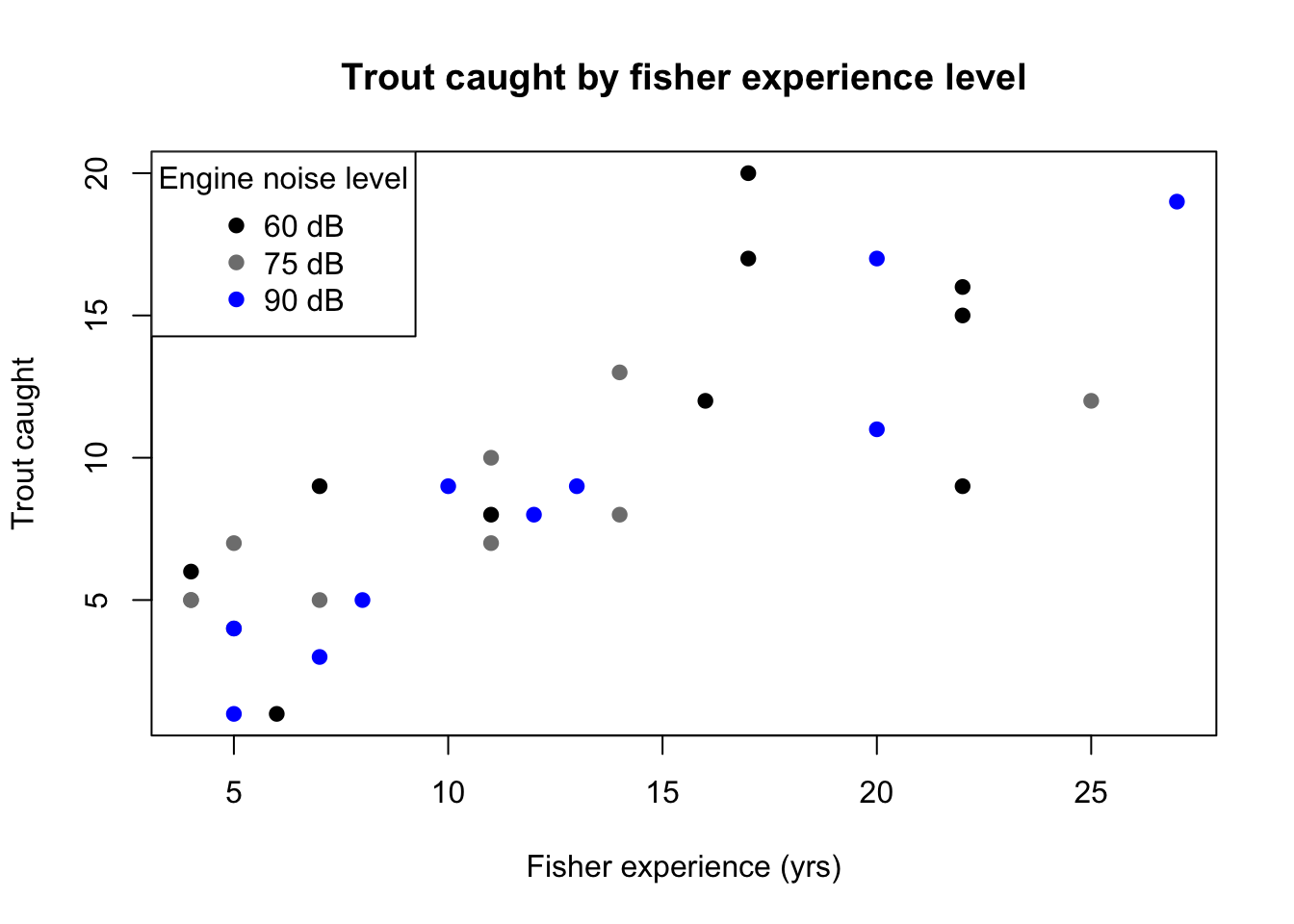
Suppose that our lake fisher starts a fishing guide business, taking boats full of experienced fishers to all the best spots in the lake. All of the tourists have fished at least a little, but the more experienced fishers often catch more fish due to their equipment, skills, and knowledge base. Another factor to consider is the motor noise: depending on the tour size, the fishing guide takes one of three boats onto the lake, and the larger boats have louder motors which might scare fish away. However, trout often swim in deeper waters farther from the motor noise, so the guide does not know if this will be an issue.
| Motor noise (dB) | 60 | 60 | 60 | 60 | 60 | 60 | 60 | 60 | 60 | 60 |
| Experience (yrs) | 13 | 19 | 4 | 6 | 6 | 14 | 17 | 8 | 18 | 5 |
| Caught | 7 | 11 | 9 | 6 | 7 | 7 | 11 | 12 | 14 | 7 |
| Motor noise (dB) | 75 | 75 | 75 | 75 | 75 | 75 | 75 | 75 | 75 | 75 |
| Experience (yrs) | 27 | 5 | 7 | 4 | 14 | 5 | 18 | 8 | 27 | 6 |
| Caught | 19 | 2 | 2 | 2 | 10 | 5 | 14 | 4 | 20 | 4 |
| Motor noise (dB) | 90 | 90 | 90 | 90 | 90 | 90 | 90 | 90 | 90 | 90 |
| Experience (yrs) | 16 | 20 | 42 | 8 | 9 | 11 | 5 | 21 | 14 | 5 |
| Caught | 8 | 10 | 21 | 0 | 1 | 5 | 6 | 16 | 8 | 4 |
The plot of the data does not strongly suggest a log-link: the middle of the response distribution seems to vary linearly with experience, and the effect of motor noise is visually uncertain. The predictors do not obviously require a log-link either: we do not think that fishers with 50 years experience can catch an amount of trout powers of ten greater than fishers with “only” 20 years experience. Contrast this to the depth data in the previous section: if trout really do prefer the deep waters, then they may be drastically less likely to be found just a few meters outside their comfort zone, and a non-linear relationship would seem justified.
The functional form of this data is simple and familiar:
\[\hat{\mu}_i = \hat{\beta}_0 + \hat{\beta}_1 \,\textrm{Experience}_i + \hat{\beta}_2 \,\textrm{Noise}_i\]
By using an identity link, we are allowing a linear combination of our predictors to directly set the center of our predicted Poisson values, just like OLS regression where a linear combination of our predictors sets the center of our expected Normal distribution. Interpreting our coefficients (the estimated betas) is also similar:
trout.identity <- glm(trout2~experience+motornoise,family=poisson(link='identity'))
summary(trout.identity)| Parameter | Estimate | p-value |
|---|---|---|
| \(\beta_0\) (Intercept) | 7.042 | 0.042 |
| \(\beta_1\) (Fisher experience) | 0.617 | <0.0001 |
| \(\beta_2\) (Engine noise) | -0.073 | 0.083 |
| \(\,\) | ||
| Null deviance | 87.695 | (29 df) |
| Model deviance | 27.015 | (27 df) |
We see from these results that a fisher with no experience, on a boat making no noise, would be expected to catch around seven trout. For each year of prior experience, their average catch size increases by about 0.6, and for every 10 dB of noise made by the boat’s motor, the catch size might be expected to decrease by 0.7 — however, this result is only marginally significant and so it would be a personal or contextual decision to include motor noise in the “final” model.
Knowing the mean of our expected counts does not provide much certainty. Even if we happened to have estimated the functional form and the betas correctly (which we have not), the actual catch amounts will be drawn from a Poisson distribution, where the variance is the same as the mean. So for larger predicted catch values we will see a wider range of catches: this does not mean we are modeling it poorly!
plot(experience,trout2,main='Predictions of Poisson identity link GLM',
     xlab='Fisher experience (yrs)',ylab='Trout caught',pch=19)
newdata <- list(experience=seq(4,27,0.1),motornoise=rep(75,231))
lines(seq(4,27,0.1),predict(trout.identity,newdata=newdata),
      lty=2,col='grey50',lwd=2)
lines(seq(4,27,0.1),qpois(0.1,predict(trout.identity,newdata=newdata)),
      col='grey50',type='s')
lines(seq(4,27,0.1),qpois(0.9,predict(trout.identity,newdata=newdata)),
      col='grey50',type='s')
legend(x='topleft',col=c('black','grey50','grey50'),lty=c(NA,2,1),lwd=c(NA,2,1),pch=c(19,NA,NA),
       legend=c('Observations','Estimated mean','Estimated 80% of outcomes'),bty='n')
The figure above shows the mean response and the middle 80% of predicted counts for every level of fisher experience, and a 75 dB motor noise assumption.
When should we choose a log link and when should we choose an identity link? Ideally, the nature of our problem will suggest an appropriate link function:
If we were predicting events of observable volcanic activity among different magma chambers and calderas, we might choose a log link. The Ideal Gas Law relates pressure, volume, amount of material, and temperature using the following formula: \(PV=nRT\) (with \(R\) being a constant). Changes in any one of these variables creates proportional changes in the others, not additive changes, and so the log link might be well-suited to the data.
If we were predicting cases of leukemia from a person’s exposure to different sources of ionizing radiation, we might choose an identity link. Current health models, while debated and contested, suggest that leukemia risk varies roughly linearly with the aggregate exposure to all sources of radiation.
If we were predicting daily crashes on a long stretch of highway, traffic density may or may not be a linear predictor for our response mean. For single-car accidents (say, tire blowouts, or failing to take a curve correctly), it is probably true that the number of crashes scales linearly with the number of cars that travel through the highway. But for multi-car accidents (say, a collision when switching lanes, or when merging onto the highway from an access road), it’s possible that they happen only very rarely below a certain traffic density and grow very quickly above that threshold. We may want to try two or more links and compare them using AIC.
Before we consider extensions to the Poisson model, I want to cover one particular proportional effect seen in many count regressions, a model offset term which enters the log link model as a predictor with a known beta of exactly 1.
We don’t often know the “true” beta for a predictor, so what is this mysterious offset term? Consider again the idea of a Poisson process: an event-generating process observed over a specific window or interval. The number of observed events is usually Poisson distributed and the time between events is usually exponentially distributed. One of the assumptions of any Poisson process is that the expected number of observed events is directly proportional to the size of the window or interval:
If we were counting annual instances of wildfires within large forests, we would expect a forest twice as large to produce twice as many fires.
If we were counting the number of buses that arrive at a bus stop, we would expect to count twice as many buses if we observed for twice as long a period of time.
If we were counting annual chicken pox cases at different elementary schools, we would expect schools with twice as many students to have twice as many cases.
The window or interval in each of these cases might be measured in units of time, or area, or people, or some other quantity, but they all can be measured and if we change this interval then the number of expected Poisson process events should scale proportionally.
Sometimes when we observe counts from a Poisson process, each observation comes from Poisson processes with different interval sizes. It would be an “apples-to-oranges” comparison if we used these different observations without any adjustment. Any difference in their counts would be wrongly attributed to differences in their predictor values when really the difference was being driven by the window size.
Let’s suppose that our fishing guide returns to the question of an ideal depth at which to fish for lake trout. They take 20 more trips out onto the lake, fishing at different depths and for different times each trip:
| Depth (m) | 10.50 | 10.50 | 10.75 | 11.75 | 12.00 | 12.25 | 12.75 | 13.00 | 13.50 | 14.75 |
| Trip time (hrs) | 2.5 | 2.75 | 2.75 | 2.75 | 2.75 | 3.50 | 3.50 | 3.75 | 4.25 | 4.25 |
| Caught | 1 | 0 | 1 | 1 | 2 | 4 | 2 | 2 | 2 | 9 |
| Depth (m) | 14.75 | 16.00 | 18.00 | 18.00 | 18.25 | 18.25 | 18.50 | 18.50 | 19.00 | 19.75 |
| Trip time (hrs) | 4.25 | 4.50 | 4.75 | 5.50 | 5.75 | 6.00 | 6.25 | 6.50 | 7.25 | 7.25 |
| Caught | 7 | 8 | 19 | 19 | 29 | 36 | 23 | 32 | 42 | 28 |
Notice that the fishing guide spends longer at the deeper fishing sites. This makes sense: they’re likely to stay longer when the fish are biting (in the deeper waters) and they’re likely to move on when nothing’s happening (in the shallow waters). So not only do we have Poisson intervals of different lengths, but also multicollinearity with our other predictor, line depth. Predictably, this would cause problems if we entered both into a log link regression, with the two predictors explaining away each other’s effects:
set.seed(1209)
(depth2 <- sort(floor(runif(20,40,80))/4))
(hours <- sort(floor(runif(20,10,30))/4))
(trout3 <- rpois(20,(hours-1)/8*exp(-1+0.25*depth2)))
trout.nooff <- glm(trout3~depth2+hours,family=poisson)
summary(trout.nooff)
exp(trout.nooff$coefficients)| Parameter | Estimate | p-value |
|---|---|---|
| \(\beta_0\) (Intercept) | -3.763 | <0.0001 |
| \(\beta_1\) (Line depth) | 0.356 | <0.0001 |
| \(\beta_2\) (Trip time) | 0.070 | 0.562 |
| \(\,\) | ||
| Null deviance | 264.935 | (19 df) |
| Model deviance | 19.162 | (17 df) |
| AIC | 97.622 |
The model above isn’t a bad model — the model deviance shows that it fits the data reasonably well. But the model is fundamentally misspecified. Trip time isn’t even found to be significant, which is clearly wrong, and the exponentiated coefficient suggests that every extra hour on the lake increases trout catch totals by 7.2%, which does not seem reasonable (additive shifts in time spent fishing should not yield proportional shifts in caught fish).
Let’s assume our doughty guide revises their initial analysis. As they think about how each fishing trip unfolds, they estimate that the first half-hour and last half-hour of most trips are not “quality fishing time”, but prep time and transit away from shore and out into the deeper lake waters. They add an offset to the linear predictor of \(\log (\textrm{time} - 1)\). Since they are using a log link, it’s necessary to log-transform the time offset so that it directly modifies the Poisson intensity, lambda:
\[\begin{aligned} \hat{\lambda}_i = \hat{\mu}_i &= e^{\mathbf{X}\boldsymbol{\beta} + \log (\textrm{time} - 1)} \\ &= e^{\mathbf{X}\boldsymbol{\beta}} \cdot e^{\log (\textrm{time} - 1)} \\ &= e^{\mathbf{X}\boldsymbol{\beta}} \cdot (\textrm{time} - 1) \end{aligned}\]
The use of an offset term has now changed our interpretation of the betas in the model. Instead of modeling the total count of the response variable, we are now modeling the rate of response counts for a single unit of the offset variable. In this example, we are now estimating the number of trout caught per hour at different line depths:
trout.off <- glm(trout3~offset(log(hours-1))+depth2,family=poisson)
summary(trout.off)
exp(trout.off$coefficients) | Parameter | Estimate | p-value |
|---|---|---|
| \(\beta_0\) (Intercept) | -3.112 | <0.0001 |
| \(\beta_1\) (Line depth) | 0.255 | <0.0001 |
| \(\,\) | ||
| Null deviance | 108.139 | (19 df) |
| Model deviance | 18.135 | (18 df) |
| AIC | 94.596 |
Notice how the coefficient for line depth has changed from 0.356 to 0.255. I actually simulated this data (and the depth data seen previously) using a true beta of 0.25, so adding an offset has helped us recover the true relationship much better than we could without the offset. Exponentiating the coefficient for line depth, we find that increasing line depth by 1 meter increases the trout/hour catch rate by 29.1%, which closely matches our earlier estimate with a previous dataset of 26.7%.
Compare the deviances in the two regression summaries printed above. The null deviance without an offset was approximately 265; with an offset, 108. By manually adjusting the counts so that they now become “apples-to-apples” rates, we have removed a large source of variation from the data, and the remaining space for modeling improvements is now smaller. We can’t perform a deviance test between the model with an offset and the model without an offset because of this difference in starting points. However, we can still compare the two models using their AICs, since there’s no change to the response variable of fish caught. By this measure, we further confirm that the model with an offset (AIC=94.6) is a better fit to the data than the model without an offset (AIC=97.6).
Remember that the Poisson distribution measures non-negative integer counts, so the mean \(\lambda\) can never be negative. Moreover, the PDF includes the term \(y!\) which is not defined for the negative values of \(y\) implied by a negative mean.↩︎
The p-value of this hypothesis test would be how often a chi-squared distribution with \(29-28=1\) degrees of freedom would generate a value of at least \(283.426-29.039 \approx 254.387\), which is essentially… never.↩︎
The p-value of this hypothesis test would be how often a chi-squared distribution with 28 degrees of freedom would generate a value of at least 29.039, which is roughly 41% of the time.↩︎