One building block of statistical time series analysis is the autoregressive (AR) model. As the name implies, an AR model presumes that past values of the series can be used to directly predict current values using a regression-like structure:
I wrote the equation above using the notation of linear regression. We will be expressing the same concept using slightly different notation below.
AR(1) process
Let’s take the simplest case, where each value of the series is predicted only by the previous value. We would name this an autoregressive model with order 1 or AR(1) model.
Note
Let \(\boldsymbol{Y}\) be a time series random variable observed at regular time periods \(T = \{1, 2, \ldots, n\}\). Let \(\boldsymbol{\omega}\) be a white noise process observed at the same time periods. If,
\[Y_t = \phi Y_{t-1} + \omega_t\]
For some \(\phi \in \mathbb{R}\) and all \(t \in T\), then we say that \(\boldsymbol{Y}\) is an autoregressive process with order 1
In theory, the exact properties of an AR(1) process depend on both the autoregressive parameter \(\phi\) as well as the specific type of white noise process denoted by \(\boldsymbol{\omega}\). In practice, we often assume \(\boldsymbol{\omega}\) to be Gaussian white noise, leaving \(\phi\) as the only input which needs estimation.
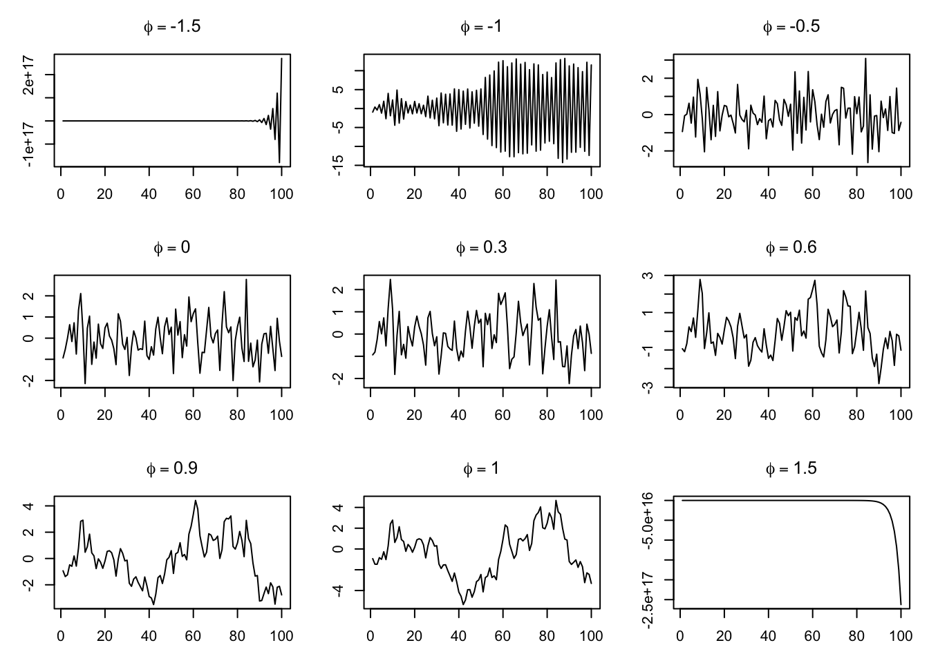
The plots above provide examples of some specific properties of AR(1) processes:
When \(\phi \gt 1\) or \(\phi \lt -1\), we say the process is explosive. After a short-to-moderate ‘fuse’, the innovations begin to cumulate exponentially, rapidly heading toward infinity.
When \(\phi = 1\), we say that the process is a random walk, since we now have the familiar model \(Y_t = Y_{t-1} + \omega_t\). When \(\phi = -1\) we have a variant on a random walk in which both the odd and even observations begin closely-related random walks headed in opposite directions.
When \(-1 \lt \phi \lt 1\) we observe a stationary process. This includes the case where \(\phi = 0\) (pure white noise), but also other series with noticeable positive or negative autocorrelation. Despite the autocorrelation, the mean and variance of the unconditional variables \(Y_t\) (that is, without knowing the past values of \(\boldsymbol{Y}\)) remain the same, and the autocorrelation of two values depends only on their lag distance, not their time index values.
Generalizing to AR(p)
Now we may complicate the scenario, by allowing the current value \(Y_t\) to have several, different relationships with arbitrary past lags of the series.
Note
Let \(\boldsymbol{Y}\) be a time series random variable observed at regular time periods \(T = \{1, 2, \ldots, n\}\). Let \(\boldsymbol{\omega}\) be a white noise process observed at the same time periods. If,
For some \((\phi_1, \phi_2, \ldots, \phi_p) \in \mathbb{R}^p\) and all \(t \in T\), then we say that \(\boldsymbol{Y}\) is an autoregressive model with orderp.
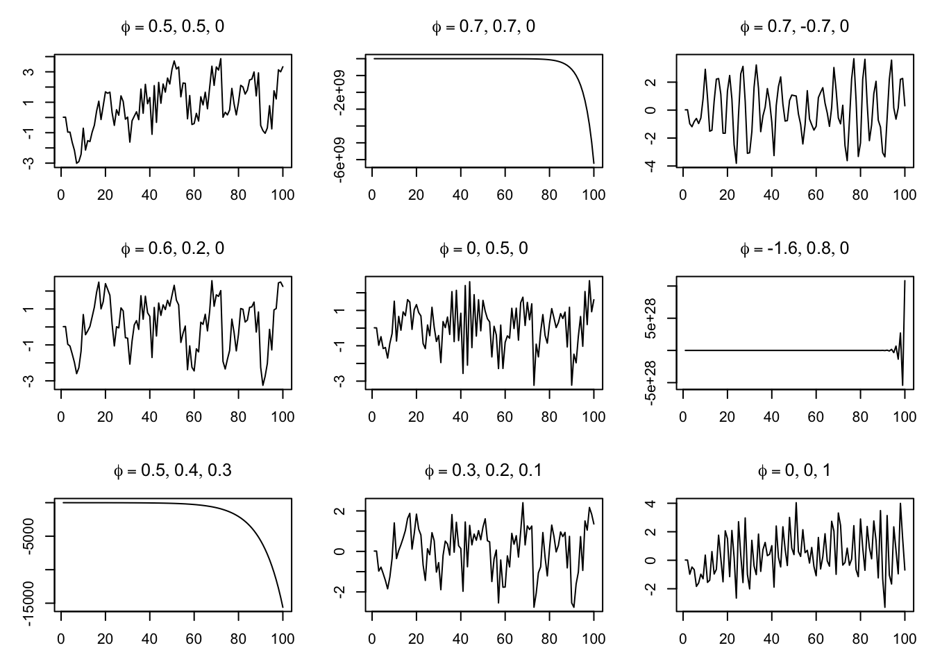
These AR(p) processes can be difficult to visually distinguish because of the more complicated autocorrelation patterns.
Nine AR(2) and AR(3) processes with the same innovations
Recognizing an AR process from its ACF plot
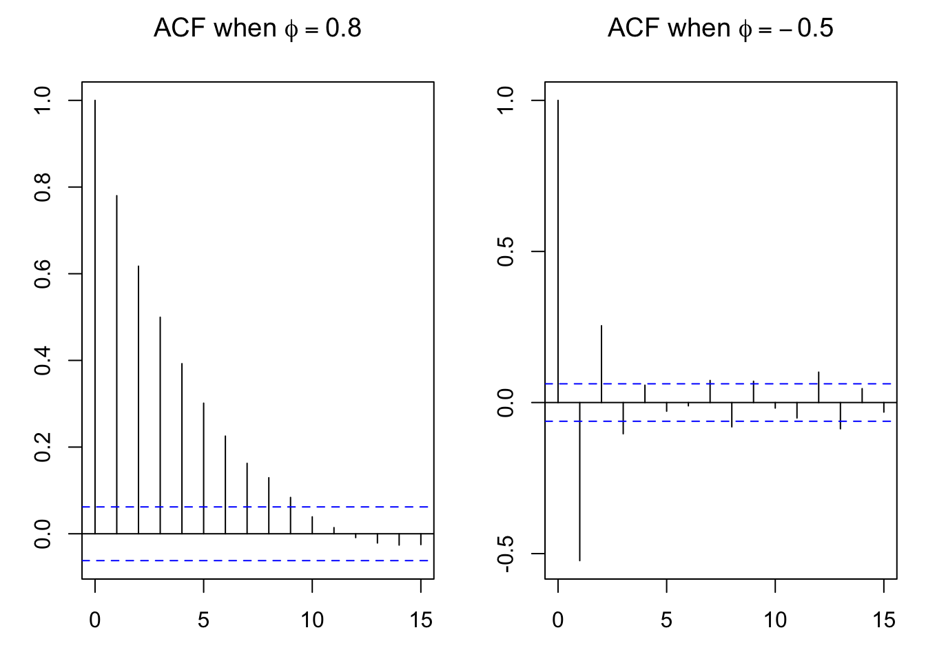
An autocorrelation function (ACF) plot will sometimes provide helpful summary or diagnostic information about an AR(p) model. In the simplest case of AR(1), the height of the ACF plot at the first lag will be equal to p, and the remaining lags will scale geometrically downward. For example, when \(\phi=0.8\), the second lag will have an autocorrelation of roughly 0.64, and the third lag will have autocorrelation of roughly 0.512
Code
par(mfrow=c(1,2),mar=c(3.1,3.1,3.1,1.1))set.seed(0108)ar08 <-arima.sim(list(ar=0.8),n=1000)arneg05 <-arima.sim(list(ar=-0.5),n=1000)acf(ar08,main=expression(paste('ACF when ',phi ==0.8)),lag.max=15)acf(arneg05,main=expression(paste('ACF when ',phi ==-0.5)),lag.max=15)
Two AR(1) processes and their ACF plots, 1000 obs each
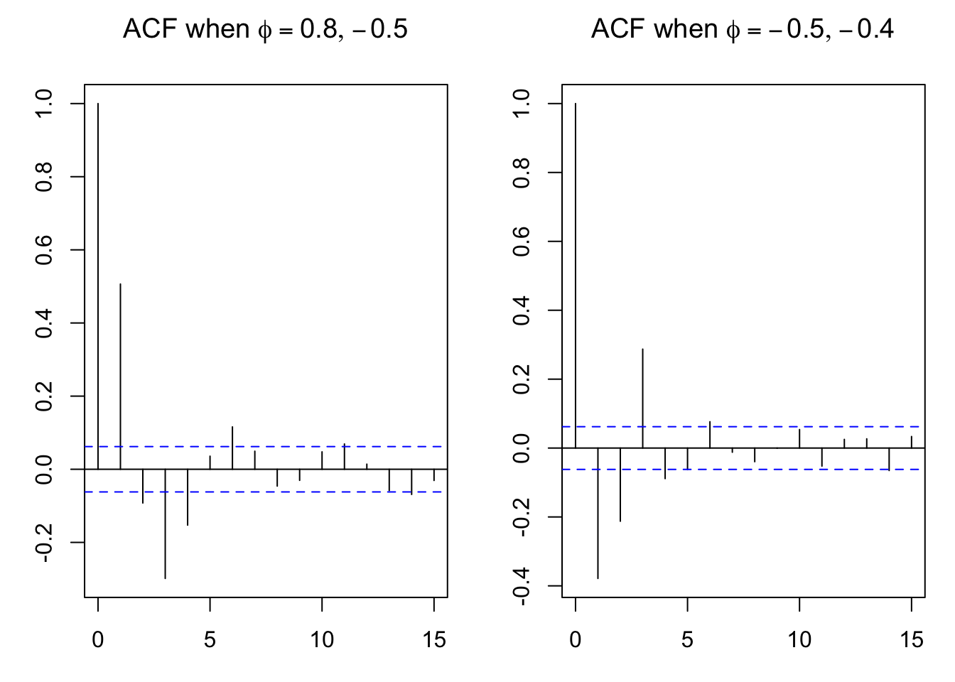
More complex AR models have correspondingly complex ACF plots, and you will not always be able to easily diagnose the order and coefficient sizes:
Code
par(mfrow=c(1,2),mar=c(3.1,3.1,3.1,1.1))set.seed(0109)ar08neg05 <-arima.sim(list(ar=c(0.8,-0.5)),n=1000)arneg05neg04 <-arima.sim(list(ar=c(-0.5,-0.4)),n=1000)acf(ar08neg05,main=expression(paste('ACF when ',phi ==list(0.8,-0.5))),lag.max=15)acf(arneg05neg04,main=expression(paste('ACF when ',phi ==list(-0.5,-0.4))),lag.max=15)
Two AR(2) processes and their ACF plots, 1000 obs each
You do not need to be able to spot a complex AR model from a brief inspection of its time series or its ACF plot. However, you should know that complex behavior can be very accurately fit by a relatively simple AR model.
Which AR processes are stationary
We will learn more about this elsewhere, when we discuss unit roots. For now, I will leave you with a simple set of guidelines:
AR(1) processes are stationary when \(|\phi_1| \lt 1\)
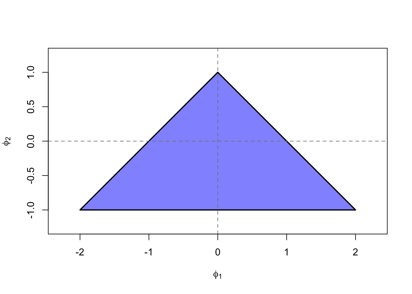
AR(2) processes are stationary when three conditions are met:
Representing the two parameters \(phi_1\) and \(\phi_2\) on the coördinate plane, we would say any process with its parameters inside the shaded region is stationary:
For AR(3) and higher processes, stationarity will depend upon the roots of the characteristic polynomial, which can be calculated with a unit root test.
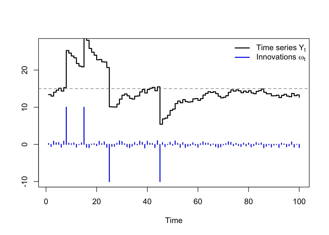
AR model responses to system shocks
AR models translate one-time system shocks into persistent, slowly-decaying signals. Consider a simple AR(1) model which processes a fairly quiet series of innovations, interrupted irregularly by a much larger signal: