Model validation refers to how we build confidence that we have constructed a model worth using to solve real-world problems. Importantly, model validation is not the same as model performance or model accuracy. A low-performance model may be the best we can reasonably fit to the data. A high-performance model may not be sufficiently better than a simple “null” model to justify its use.
Time series models can be used simply to understand the past, much like cross-sectional techniques such as linear regression. However, when time series models are used specifically to forecast the future, we need to be very wary of in-sample performance on the training data. After all, the whole point of forecasting is out-of-sample prediction, so we should try to understand the model’s out-of-sample performance as best as we can.
Backtesting your model
As compared to ordinary cross-validation
Non-time series models frequently use cross-validation to build confidence in the models. (In cross-validation, the training data is split into \(k\) blocks of roughly equal size, and each block is used as a test dataset for a model trained on the remaining \(k-1\) blocks.)
We can’t use this technique in time series analysis because it cannot preserve the time indexing of the data, which in turn affects our model predictions. Having a block of observations missing from the middle of our data is often enough to “break” our model, and in any case to predict for these points would involve using future information to predict the past, which would not validate our model usefulness.
Time series cross-validation
One best practice which implements cross-validation concepts for time series modeling is called, plainly enough, time series cross-validation. (Sometimes this technique is also called “backtesting”, though backtesting could also refer to less formal methods or simply a single prior validation period.)
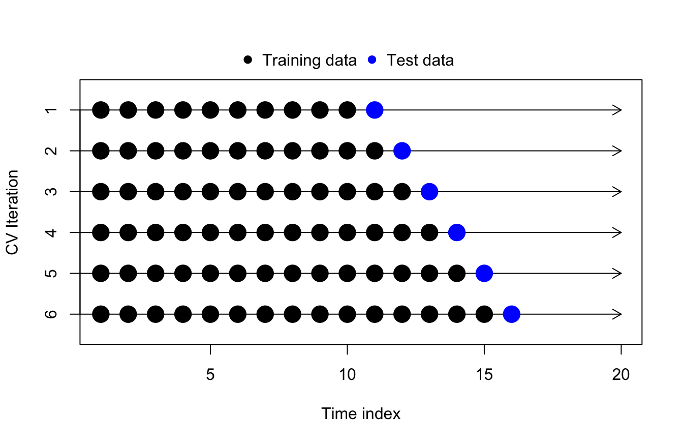
The basic idea of time series cross-validation is to forecast each observation in our training data (as far back as practical while retaining enough of a prior training sample), and after each forecast is complete we then incorporate that observation into our training set for the new data:
Once we have forecasted as much of the training data as possible through time series cross-validation, we can compute out-of-sample performance metrics such as MAE or RMSE by aggregating across the test forecasts.
Variations on basic time series cross-validation
As a forecaster (and more generally as a data scientist), you must do more than simply memorize how to drop a pre-written routine into your workflow: you will need to know how to choose and adapt a technique to the problem that you’re solving. As an example, consider three variations on the basic timeseries cross-validation method described above.
Fixed-width training windows
Some models avoid parameter drift by de-weighting old observations (e.g. ETS, neural networks), while other models avoid parameter drift by avoiding parameters altogether (e.g. KNN). When using these models, the dangers of inlcuing stale training data are largely minimized.
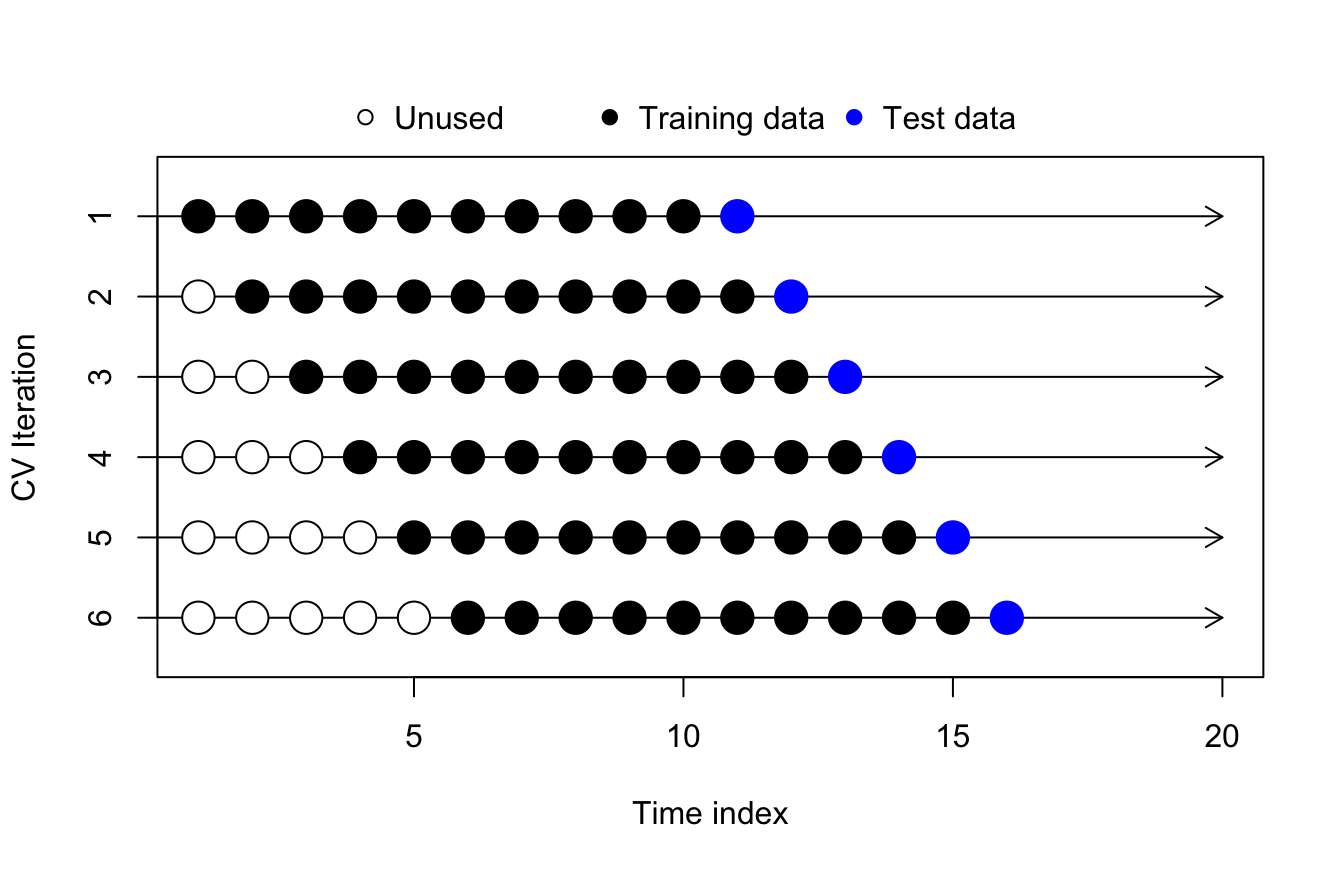
Other models, like ARIMA models, VARs, or dynamic regressions, equal-weight the entire training range and are sensitive to parameter drift or structural breaks. When running these models over a large amount of data, you might want to limit the size of the training sets used for time series cross-validation, to more accurately reflect the limited training datasets you intend to provide your model “in production”:
Time series cross-validation with fixed-width training windows
As an example, econometricians and legal experts sometimes analyze daily securities prices (stocks, hedges, commodities, futures, options, etc.) using time series models. A greater amount of training data (prior daily prices) helps to better estimate the model, but too much data runs the risk of parameter drift, structural break, or contaminating the sample with otherwise outdated information. In most literature, one year of daily price returns is seen as a good compromise, with six months or two years being common alternatives. The basic cross-validation procedure might involve fitting models with 10+ years of training data, which is not how these models would ever be used in practice.
Cross-validating h-ahead forecasts
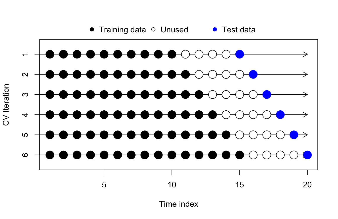
In some instances, the one-ahead forecast is not an organizational priority, but forecasting on a longer time horizon is more valuable. A realtor or a bond market trader may want to gain insight into the expected interest climate next year, not just next quarter. In these cases, we should match our validation to the forecast window(s) which will be used for decision-making, even if the metrics for the one-ahead forecast period are stronger (which will almost always be true):
Depending on the problem and the organizational interest in solving said problem, multiple forecasting horizons might be important to understand. The same forecasting methods for interest rates could be validated at a 1-month, 12-month, and 60-month horizon. Different models could be chosen for each horizon, or a model could be chosen which performs as well as possible across all three horizons simultaneously, depending on the user’s needs and preferences.
(Note that a direct forecasting approach naturally dovetails with the idea of validating each time horizon separately, while a recursive forecasting approach naturally suggests itself when choosing one model to be “good enough” at all horizons of interest.)
Cross-validating MIMO forecasts
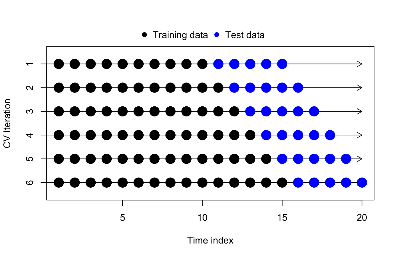
Time series cross-validation extends simply to MIMO forecasts, though even here we may find nuance and user judgment calls. For example, say I were a meteorologist tasked with five-day forecasts (of daily weather, or perhaps the track of a hurricane). I could train a five-day MIMO model, and I could cross-validate it by rolling the training window through my data one day at a time:
Time series cross-validation of 5-day MIMO forecasts
Even though the test regions overlap, this setup would provide perfectly acceptable validation of my model! In fact, by allowing the test windows to overlap, we preserve crucial details about the dependence structure. If we tested only the observations \(y_{11}, \ldots, y_{15}\) as one iteration and then the observations \(y_{16}, \ldots, y_{20}\) as the next iteration, we would never ask our model to incorporate both \(y_{15}\) and \(y_{16}\) in the same test period. That particular transition might be extreme or unexpected; failing to test it could obscure weaknesses in our model.
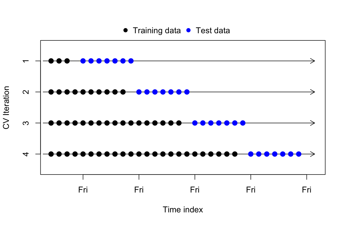
However!! What if, instead, I worked as a grocery store manager. Each Wednesday I place my orders with suppliers to restock my store Friday morning ahead of the weekend rush. If I have to resupply midweek I can, but I need to know ahead of time, and if I order too much food it may end up as costly spoilage.
In this situation, it would be more appropriate to slide the training window one week at a time, predicting each future week’s sales Friday to Thursday. We have no current use for a model which predicts grocery sales Tuesday to Monday. (Though we did have a use for a hurricane forecasting tool which could be used every day.)
Time series cross-validation of 7-day MIMO forecasts
Choosing a model
Validation is one part of a multistep process which ends with our adoption of a forecasting model. Let’s examine the other parts to see how validation contributes to the final decision.
1. Identify the status quo
In some organizational settings, a forecasting model is already in place, and you are asked (or you are offering) to improve upon it.
If the existing codebase and data is available to you, start by using the exact model, on the real data.
If you simply have a description of the status quo, replicate the model and the data as best as you can. Even small details can create large changes in forecast accuracy, so treat this step very carefully.
In other settings, your model will be the first used to address the business problem or research question.
Determine the best “null model” and its associated forecast method which would make sense for this application. Depending on the problem, a null model might be a random walk (where the forecast is the last observed value), white noise (where the forecast is the mean of the historical data), linear regression (no true interdependency, just extrapolation using a time-based covariate), etc.
Use the status quo or the null model to prove the worth of your work. If your modeling efforts do not meaningfully surpass the status quo, then you should stop the analysis. Do not see this outcome as a personal failure or an unsuccessful project. Instead, you will be saving your organization the cost (in money and time and risk) of changing forecast methods, and delivering new knowledge to decisionmakers about the ability or inability to meaningfully predict the future of this data series.
2. After EDA, pick a very limited number of contenders
Students and junior professionals often mistakenly select many different models and run them against each other to “prove” they have found the right approach. Usually, they achieve the opposite result:
By selecting models which are not well-fit to the problem, they suggest either domain inexperience or data science inexperience,
By selecting many different models, they rarely give proper attention to each, in terms of the feature engineering or hyperparameter tuning they would realistically require.
By selecting many models, they make it more difficult to communicate their work to others and have it be easily understood and trusted.
By selecting many models, they increase the chance of overfitting the problem and seeing much worse performance in production than during testing.
By selecting many models, they increase their own workload and place needless strain on their deadlines.
Instead, aim to exit this step with one or two classes of model, perhaps with one or two variants each. Choose models that fit the problem: don’t bring an ARIMA model to a GARCH problem, or choose a neural network model (RNNs, LSTMs) with inputs which fail to capture the long-period seasonality in your data.
In other words, confirm the functional form of your model candidates through EDA. Do not use extensive model validation simply to show that an AR representation fits the data better than an MA representation: you can and should do this without time series cross-validation. Only bring true contenders to the validation phase.
3. Pick a forecasting method and one or two metrics to help you evaluate the models both in absolute and relative terms.
At this point you will be choosing between the status quo model (the “champion”) and one or two new models which have been fully built out and polished. If those models involve tuning parameters or other hyperparameters, then ideally these choices will have already been set using additional training data different than the validation training set.1
Which forecast method will you use? Generally, there will only be one right choice, fitted to your model type(s) and business problem, though occasionally you may simultaneously test the models over multiple time horizons.
Which metric will be computed from the time series cross-validation?
Root mean squared error (RMSE): The classic. Heavily penalizes large errors. Often described as the size of an “average” error although this is not mathematically true. Some models minimize the in-sample RMSE by construction, so it’s a fitting comparison to see how they perform out-of-sample.
Mean absolute error (MAE):Actually the size of the “average” error. Does not disproportionally penalize large errors. Most useful when errors are naturally and tightly bound (e.g. when predicting proportions), or when the large errors are not particularly costly (e.g. when predicting future daily wind speed).
Mean absolute percentage error (MAPE): A metric which solves some problems but introduces others. Unitless, and therefore good for measuring predictions which vary wildly in their mean as well as comparing models trained on different datasets or different periods. However, the metric does not handle values near zero very well and it assigns an asymmetrically larger penalty to negative errors as compared to positive errors.
Mean absolute scaled error (MASE): Introduced by Hyndman and Koehler, solves many problems with MAPE. Benchmarks the challenger model’s forecast errors using the errors from a naive “null model”.
Custom cost function or value function: Often overlooked by data scientists. When you can estimate this function, it will generally be more useful than any of the above model metrics. Examples would be the costs of spoiled overage or empty shelves at a grocery store (as opposed to the forecast error in estimated demand), or the market value of an RMBS security (as opposed to the forecast error in the default rate on the underlying mortgages).
Your goal when choosing these metrics is to simultaneously learn (and communicate) whether any given model is (a)better than other models, and (b) acceptably good enough to be put into production. Both relative and aboslute performance are important.
It helps to have a goal post set before you begin validation, perhaps even before you begin modeling. What is a useful level of forecasting performance? Where is the benchmark for “worth organizational resources”? Check in with your stakeholders. Giving them the best model is not helpful when even the best model simply isn’t very good.
4. Be prepared to defend your model on its other strengths and weaknesses beyond the validation metrics
The world does not stop what it’s doing and bow down to you for achieving a remarkable forecast accuracy, sad to say. There may be skeptics among your audience or stakeholders. In fact, there should be skeptics, or at least those who will only be persuaded by a body of evidence, or else you run the risk of pushing bad models into production which have not survived legitimate scrutiny. Invite the toughest critic you know (and who is allowed to see your model) to kick the tires on your work.
You will likely be asked about some or all of the following model properties, so you should do whatever work you can to prepare for these types of questions:
How does this model fit in with the previously accepted or previously used theory? If it differs, why does it differ, and is this reasonable? If it uses the same model class as the status quo, why did the small differences in specification create large differences in model performance?
How does this choice of model characterize the world? What does it say about the underlying number generating process, and is that a statement which your organization would feel comfortable supporting? For example, are you saying that prices are not random walks? Are you saying that crime is best predicted through racial demographics?
Do the residuals or estimated innovations suggest that you have underfit the model? If any structure remains — non-stationarity, autocorrelation structures, volatility clustering, etc. — then likely you have missed a modeling opportunity which others might observe and point out to your audience.
How would you persuade someone that you have not overfit the model, through cherrypicking, “throwing spaghetti at the wall and seeing what sticks” (using many model classes and variants), information leakage, or other sources?
How resource-intensive is your model, in terms of deployment time, runtime, compute and storage requirements, employee skill sets needed for maintenance and model refreshes, data engineering tasks, etc.?
Do you like your model? Why or why not? Do you trust your model? Why or why not?
If need be, the rolling training window can include a short tuning sequence before each true test forecast(s). After using the tuning sequence to set the hyperparameters, the model is fixed in place: the tuning sequence enters the embedding horizon for the forecast without altering the training model.↩︎