Stationarity

library(fable)
library(fabletools)
library(tseries)

Motivation

We can’t perfectly forecast everything (or anything!), but perhaps we can draw a meaningful distinction between two different scenarios:

Scenario 1: The time series is inherently unpredictable. We may be able to guess that the next observation will be somewhere near the current observation, but further into the future we have no idea “where to look” for the time series.
Scenario 2: The exact values of the time series may be random, but the likely future values of the time series are estimable and the further into the future we look, the more consistent our estimates will be.

It would be nice to define these two scenarios more precisely, and to develop a test which can help us to identify which scenario we face, and perhaps even to develop techniques which transform the first scenario into the second.

Definitions

We will call the concept discussed in Scenario 2 above stationarity, which is meant to suggest that the time series “stays in place” over time. It may fluctuate, perhaps severely, but will always stay in the neighborhood of “home base”.

There are two common definitions of stationarity: we say that a time series is either strongly stationary or weakly stationary (or, of course, nonstationary).

Strong stationarity

When a time series is strongly stationary, its joint unconditional distribution does not depend on the time index. This is a bold assertion and difficult to test, but when true it unlocks many theoretical results and properties.¹

Note

Let \(\boldsymbol{Y}\) be a time series random variable observed at regular time periods \(T = \{1, 2, \ldots\}\). Let \(F_\boldsymbol{Y}\) be the joint cumulative distribution function of a set of random observations \(Y_1, Y_2, ...\) from the time series \(\boldsymbol{Y}\). Then if

\[F_\boldsymbol{Y}(Y_1 \le y_1, \ldots, Y_n \le y_n) = F_\boldsymbol{Y}(Y_{1+k} \le y_1, \ldots, Y_{n+k} \le y_n)\]

For all \(k \in \mathbb{N}\) and all \(n \in \mathbb{N}\) and all real values of \(y_1, \ldots, y_n\), then we say that the time series \(\boldsymbol{Y}\) exhibits strong stationarity.

Essentially, until we begin to actually observe values from a strongly stationary process, the probability distribution of all future points is the same, and any serial dependence between a set of observations is shared between all sets of observations with the same relative time-orderings. (For example, \(F_\boldsymbol{Y}(Y_3|Y_1=c)\) = \(F_\boldsymbol{Y}(Y_8|Y_6=c)\).)

Weak stationarity

Knowing or estimating the full joint distribution of a set of time series observations seems like a lot of work. For many purposes, we may accept a slightly looser definition of a stationary process without losing the mathematical results and guarantees we need to perform our analysis.

Note

\[\begin{aligned} (1) & \quad \mathbb{E}[Y_t] = \mu \qquad \forall \, t \in T \\ \\ (2) & \quad \mathbb{V}[Y_t] = \sigma^2 \lt \infty \qquad \forall \, t \in T \\ \\ (3) & \quad \textrm{Cov}(Y_s,Y_t) = \gamma_{|t-s|} \qquad \forall \, s,t \in T\end{aligned}\]

Then we say that the time series \(\boldsymbol{Y}\) exhibits weak stationarity.

Weak stationarity makes fairly straightforward claims about the first and second moments of \(F_\boldsymbol{Y}\) rather than trying to define its entire joint distribution. Constant mean, constant and finite variance, and an autocovariance function which depends only on the time interval between two random observations.

Non-nested definitions

Confusingly, neither strong stationarity nor weak stationarity imply the other. While it is often true that strongly stationary processes are also weakly stationary, exceptions can be found:

If \(Y_t \stackrel{iid}{\sim} \textrm{Cauchy}\) for all \(t \in T\) then the variance of each observation \(Y_t\) and the autocovariance between observations \(Y_s\) and \(Y_t\) will be undefined or infinite, meaning that \(\boldsymbol{Y}\) cannot be weakly stationary — but since the distribution is known and identical across all time indices, \(\boldsymbol{Y}\) is strongly stationary.
If \(Y_t \stackrel{iid}{\sim} \textrm{Exponential}(1)\) for odd values of \(t\) and \(Y_t \stackrel{iid}{\sim} \textrm{Poisson}(1)\) for even values of \(t\), then the mean and variance of each observation \(Y_t\) would still be 1, and the covariance between the (independent) observations would be 0, meaning that the covariance does not depend on the time indices: \(\boldsymbol{Y}\) would be weakly stationary. However, since (for example) \(F_\boldsymbol{Y}(Y_1,Y_2) \ne F_\boldsymbol{Y}(Y_2,Y_3)\), the process is not strongly stationary.²

However, these are edge cases. Importantly for our future work, a Gaussian white noise process is both strongly and weakly stationary.

Equally important, a random walk is never stationary.

Recovering stationarity from non-stationary processes

Although most time series are not stationary, we can often apply simple transformations to regain stationary behavior. I will quickly describe three examples below:

Trend stationarity

Sometimes a process is observed with a deterministic trend, that is, a steady drift of the mean away from its initial condition. If the drift in each period \(t\) is nonrandom, and known or estimable, we can remove the trend and the “de-trended” series which remains may be stationary.

Note

Let \(\boldsymbol{Y}\) be a time series random variable observed at regular time periods \(T = \{1, 2, \ldots\}\). Let \(\mathbb{E}[Y_t] = \mu + \delta t\), let \(\mathbb{V}[Y_t] = \sigma^2 \lt \infty\), and let \(\textrm{Cov}(Y_s,Y_t) = \gamma_{|t-s|}\) for all \(s,t \in T\).

Then \(\boldsymbol{Y}\) is a trend-stationary time series, and if \(X_t = Y_t - \delta t\) then \(\boldsymbol{X}\) is a weakly stationary time series.

The intuition here is quite simple: if we know or can estimate a non-random component of our time series which moves the mean (destroying stationary), then we can simply remove it when we want to study the random time series behavior and add it back in when we need to perform prediction.

Code

par(mfrow=c(1,2),mar=c(4, 4, 3, 1))
set.seed(1229)
tsts <- 70 + 3*arima.sim(list(ar=c(0.5,0.25)),n=100) - 0.4*(1:100)
plot(tsts,ylab='Y_t',main='Original data series')
abline(70,-0.4,col='#bbbbbb')
plot(tsts +  0.4*(1:100),ylab='Y_t - 0.4t',main='Detrended data series')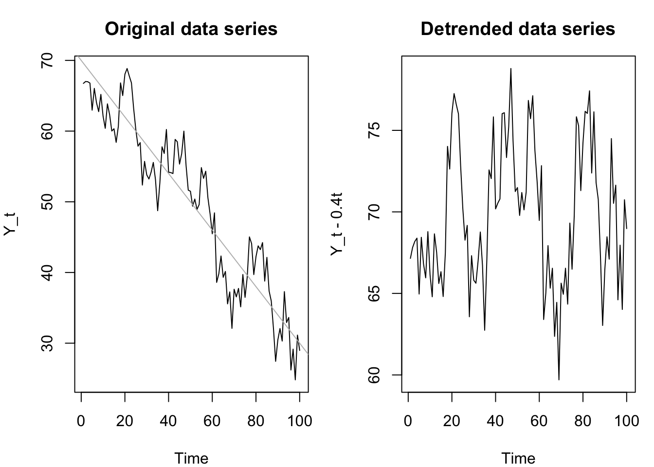

Trend-stationary process with and without detrending

Although the deterministic trend described here is additive, this concept generalizes to multiplicative trends or other situations, such as a variance which shrinks or grows at a steady rate over time.

Difference stationarity

When a time series drifts away from its mean through a stochastic (i.e. random) process, then simply “tilting” the series by removing a linear trendline will not be enough to restore stationarity.

In some cases, the differences between the values of a nonstationary series can themselves be a stationary series. The most well-known example of this is a random walk. Since the random walk is created by cumulating a white noise series, the difference of the random walk is simply the same white noise series, and a white noise series is stationary.

We now have cause to introduce the backward difference operator \(\nabla\).

\[\nabla Y_t = Y_t - Y_{t-1}\]

\[\nabla_{\!k} Y_t = Y_t - Y_{t-k}\]

Note

Let \(\boldsymbol{Y}\) be a time series random variable observed at regular time periods \(T = \{1, 2, \ldots\}\). Let \(\mathbb{E}[\nabla Y_t] = \mu\), let \(\mathbb{V}[\nabla Y_t] = \sigma^2 \lt \infty\), and let \(\textrm{Cov}(\nabla Y_s,\nabla Y_t) = \gamma_{|t-s|}\) for all \(s,t \in T\).

Then \(\boldsymbol{Y}\) is a difference-stationary time series, and if \(X_t = \nabla Y_t\) then \(\boldsymbol{X}\) is a weakly stationary time series.

Many real-life processes are essentially random walks and their levels are difficult to study, but their differences (additive or proportional) are useful targets for our analysis. One example woudl be stock prices: the growth of a company’s value over time, combined with the changing scale caused by inflation, and the complications caused by stock splits, dividends, new share issuances, and stock buybacks all combine to make the price of a stock relatively uninteresting to market analysts. However, the percentage price return, or daily proportional change, is a fundamental unit of analysis which we may model as being trend-stationary (the deterministic trend being the risk-free rate).

Knowing when to de-trend and when to difference is important. A random walk may appear to have a roughly linear trend, but the de-trended series will still be nonstationary:

Code

par(mfrow=c(1,2),mar=c(4, 4, 3, 1))
n <- 200
set.seed(1230)
rw <- cumsum(rnorm(n))
plot(rw,ylab='Y_t',main='Original data series',type='l')
lines(x=c(1,n),y=c(rw[1],rw[n]),col='#bbbbbb')
plot(rw-(1:n)*(rw[n]-rw[1])/(n-1),ylab='Y_t - Avg Drift',main='Detrended data series',type='l')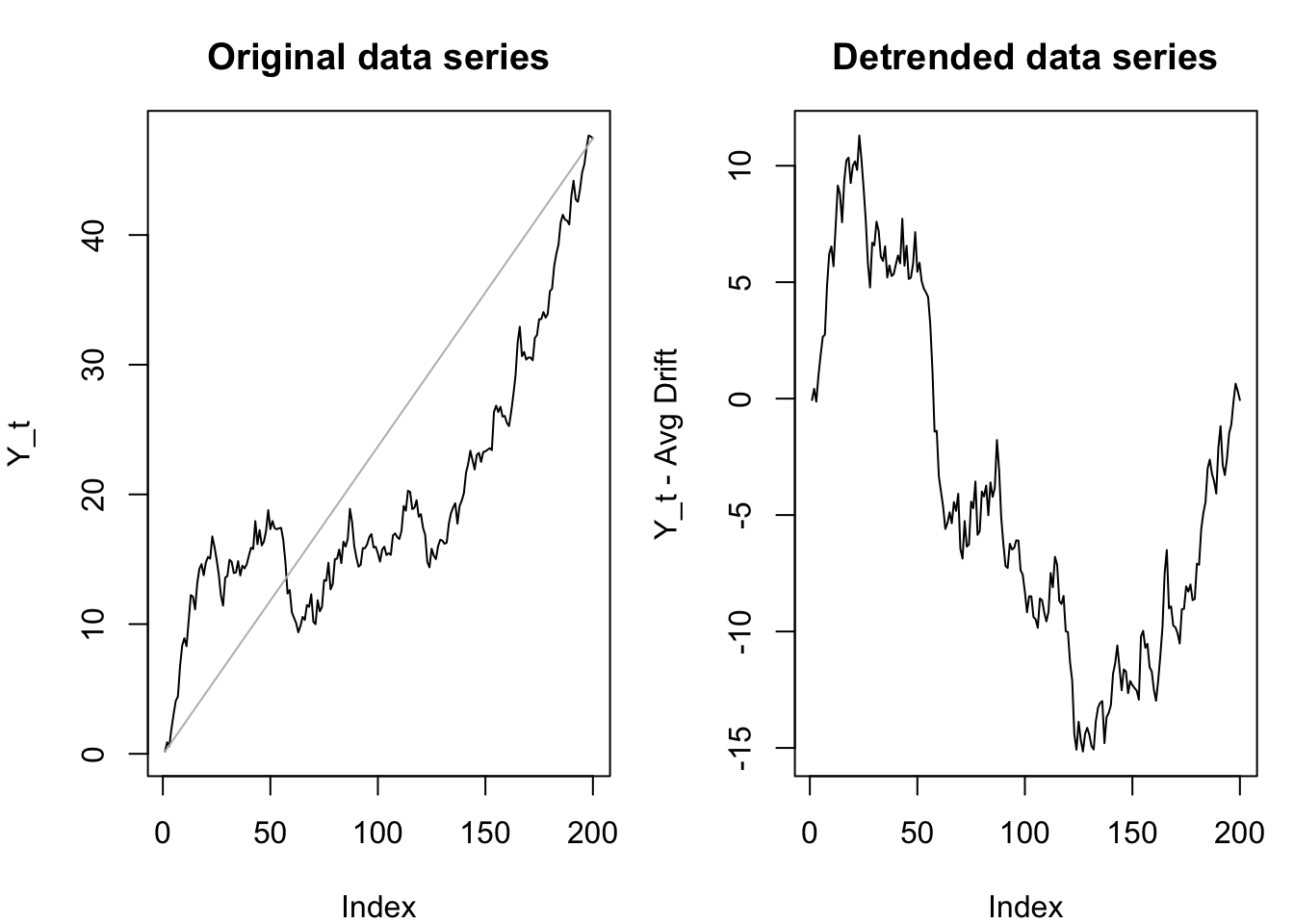

Random walks de-trended (top) and differenced (bottom)

Code

plot(rw,ylab='Y_t',main='Original data series',type='l')
segments(x0=2:n,x1=2:n,y0=0,y1=diff(rw),col='#bbbbbb')
plot(diff(rw),ylab='First difference of Y_t',main='Differenced data series',type='l')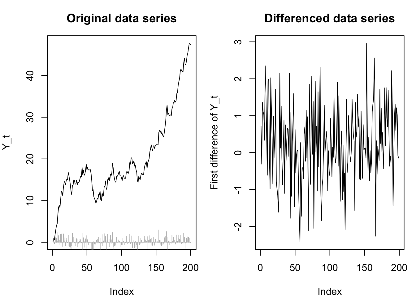

The Box-Cox transformation

In still other cases, the problem with achieving stationarity is that some growth or shrinkage over time effectively places different parts of the time series on different scales. The S&P500 index did not move by more than 5 units per day for its first 20 years… nowadays, it moves by more than 5 almost every day. Its starting value was near 50… nowadays, its value is near 5000. Both the mean and the variance have shifted over time. A special class of transformation can bring series like this closer to stationarity:

Note

Let \(\boldsymbol{Y}\) be a time series random variable observed at regular time periods \(T = \{1, 2, \ldots\}\). Define \(\boldsymbol{Y}^{(\lambda)}\), the Box-Cox transformation of \(\boldsymbol{Y}\) as follows, for any choice of parameter \(\lambda \in \mathbb{R}\):

\[Y_t^{(\lambda)} = \left\{\begin{array}{ll} \log Y_t & \textrm{if}\; \lambda = 0 \\ \frac{Y_t^\lambda - 1}{\lambda} & \textrm{if}\; \lambda \ne 0 \end{array}\right\}\]

The exact parameter \(\lambda\) which brings a nonstationary series closest to stationarity must be estimated through algorithmic means, including (but not limited to) maximum likelihood estimation. As an example below, a Box-Cox transformation with a parameter of 0.1 takes this highly nonstationary airline data and transforms it into something much closer to trend-stationarity.³

Code

data(tcm)
yields <- window(tcm1y,end=1982.24)
par(mfrow=c(1,2),mar=c(4, 4, 3, 1))
plot(yields,ylab='1Y yield',main='Original nonstationary series')
plot(box_cox(yields,0.15),ylab='Transformed series',main='Box-Cox with lambda=0.15')
abline(reg=lm(box_cox(yields,0.15)~time(yields)),col='#bbbbbb')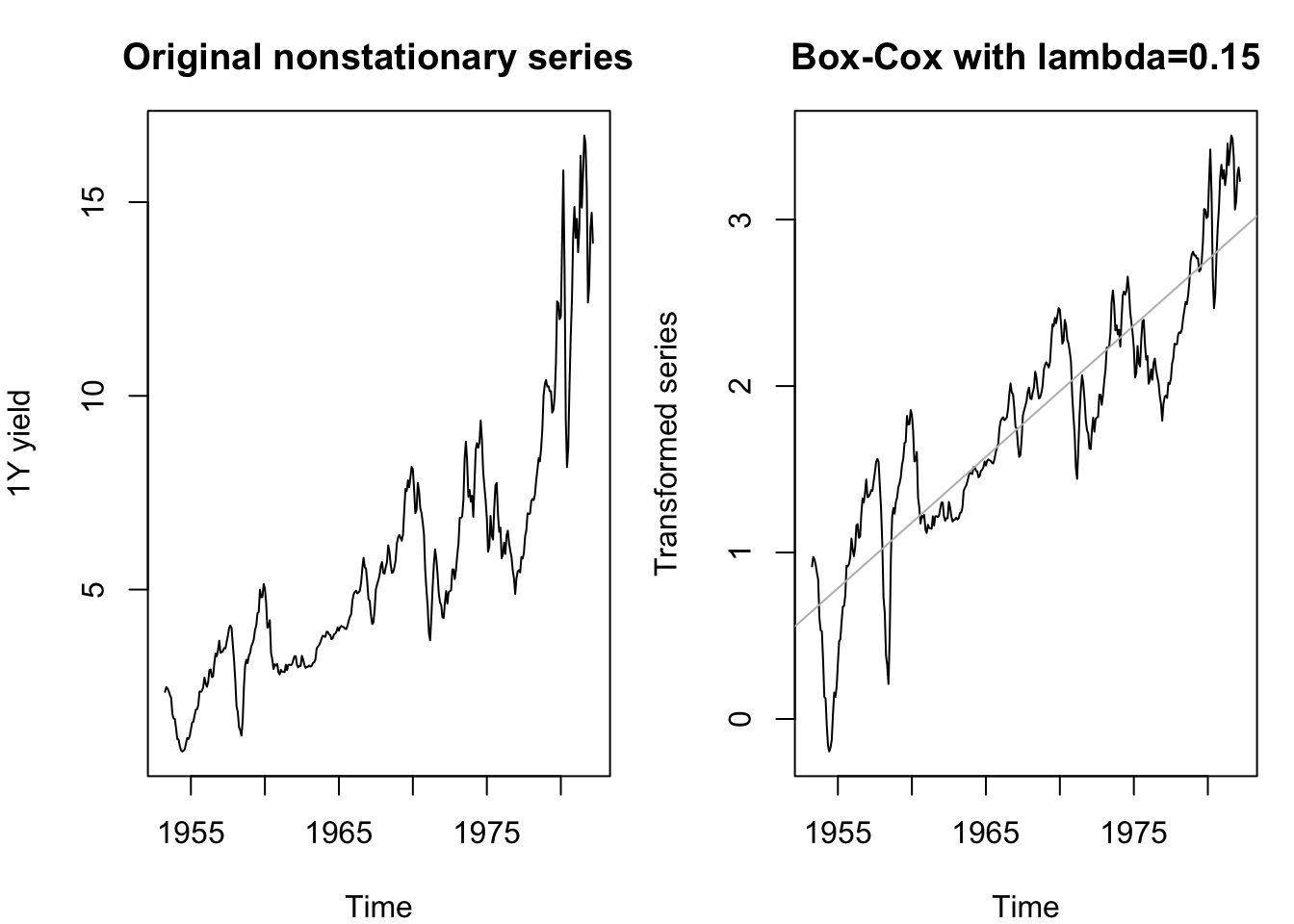

Box-Cox transformation of monthly 1Y Treasury yields

Tests for stationarity

How do we know if a series is stationary? Well, the short answer is, we don’t:

A statistical test would not prove that a series is stationary or nonstationary, only provide some degree of evidence against the null hypothesis.
Even if a time series seems stationary for the period in which we observe it, we have no guarantee it will remain stationary in the future.

Even so, optimistic statisticians have developed several tests for stationarity. Although the mathematics behind these tests is within the reach of most readers, I will focus on just two tests and discuss how they are used rather than how they are calculated.

The augmented Dickey-Fuller (ADF) test

The Dickey-Fuller test (1979) examines whether a time series might actually be a random walk or stationary (including trend-stationary). The specific model being tested is whether

\[\nabla Y_t = c + \alpha Y_{t-1} + \omega_t\]

If \(\alpha=0\) then we have a random walk with a deterministic trend: the step size between every pair of observations of \(\boldsymbol{Y}\) are a constant (creating drift) plus white noise (creating the random walk).

Because of this setup, the null hypothesis of \(\alpha \ge 0\) codes for nonstationarity, while the one-sided alternative hypothesis is stationarity (since negative values of \(\alpha\) create a “rubber band” mean-reverting process).

The augmented Dickey-Fuller (ADF) test extends this concept to control for complex autocorrelations in the original data series which might obscure the presence of a random walk. While the ADF test is slightly less powerful than the original Dickey-Fuller test, it’s more widely used today and considered an improvement upon the original.

We see that the original air passenger data series shown above fails to display stationarity, while the Box-Cox transformation does show stationarity using an ADF test:

adf.test(yields)


    Augmented Dickey-Fuller Test

data:  yields
Dickey-Fuller = -1.7333, Lag order = 7, p-value = 0.6893
alternative hypothesis: stationary

adf.test(box_cox(yields,lambda=0.15))


    Augmented Dickey-Fuller Test

data:  box_cox(yields, lambda = 0.15)
Dickey-Fuller = -3.4646, Lag order = 7, p-value = 0.0463
alternative hypothesis: stationary

The Kwiatkowski-Phillips-Schmidt-Shin (KPSS) test

The ADF test is useful and widely accepted, but carries one drawback: even when applied to truly stationary data, it often fails to reject the null hypothesis of a random walk. This created an opening for a newer test which makes stationarity the null hypothesis.

The Kwiatkowski-Phillips-Schmidt-Shin (KPSS) test proceeds by assuming that every time series can be decomposed into three parts: a deterministic time trend, a stationary error process, and a non-stationary random walk with some unknown variance:

\[Y_t = \delta t + r_t + \varepsilon_t\]

Where \(r_t\) is a random walk with variance \(\sigma^2\), and \(\varepsilon_t\) is a stationary error process.⁴

The KPSS test examines whether the random walk variance could be 0 (in which case it is not really present at all). By testing \(\sigma^2 = 0\), it creates a null hypothesis of stationarity and a one-sided alternative hypothesis that \(\boldsymbol{Y}\) is a random walk.

We see that the original air passenger data series shown above fails to display stationarity, while the Box-Cox transformation does show stationarity using a KPSS test:

kpss.test(yields,null='Trend')

Warning in kpss.test(yields, null = "Trend"): p-value smaller than printed
p-value


    KPSS Test for Trend Stationarity

data:  yields
KPSS Trend = 0.42815, Truncation lag parameter = 5, p-value = 0.01

kpss.test(box_cox(yields,lambda=0.15),null='Trend')


    KPSS Test for Trend Stationarity

data:  box_cox(yields, lambda = 0.15)
KPSS Trend = 0.14306, Truncation lag parameter = 5, p-value = 0.05544

So what have we gained, since these results are the same as the ADF test results above? Essentially, by using both tests, we can now differentiate between three distinct situations:

Compelling evidence for stationarity: The ADF and KPSS tests agree on stationarity.
Compelling evidence for a random walk: The ADF and KPSS tests agree on random walk.
Not enough evidence and power to be sure: The ADF test cannot reject a random walk but the KPSS test cannot reject stationarity.

Recall that the definition below is for regularly-observed, one-dimensional discrete time series processes. There are broader definitions of stationarity which generalize to other situations.↩︎
Consider that \(Y_1\) cannot be 0 while \(Y_2\) can with probability \(1/e\).↩︎
The seasonal peaks are nonstationary behavior, but we will learn to model these too in future lesson.↩︎
We do not use the notation \(\omega_t\) since the error process need not be white noise.↩︎