SARIMA models

library(forecast,quietly=TRUE)
library(MASS,quietly=TRUE)
library(tseries,quietly=TRUE)

We have already seen several datasets which display moderate or severe seasonality, but the ARIMA models presented earlier did not explicitly model that seasonality. We can now add that functionality to the basic ARIMA structure, creating a type of ARIMA model often known as seasonal ARIMA or SARIMA.

Motivation

Let’s say that we are looking at a new monthly time series for the first time, and try to analyze it using the Box-Jenkins ARIMA modeling approach. The first five years of a ten-year dataset are plotted below:

set.seed(0120)
y <- 2+ arima.sim(model=list(ar=c(0.5,rep(0,10),0.3)),n=120)
plot(y[1:60],type='l',ylab=expression(Y[t]),ylim=c(0,6))  
abline(v=0.5+12*(1:4),lty=2,col='#7f7f7f')
text(x=12*(0:4),y=0.1,labels=paste('Year',1:5),pos=4,col='#7f7f7f')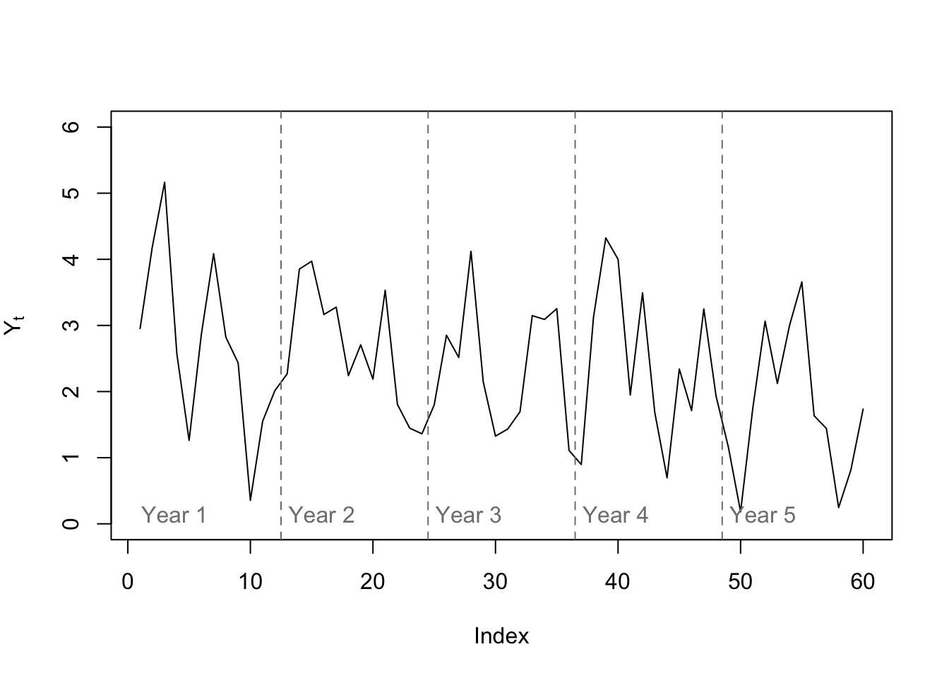

First five years of a seasonal time series

Even upon a quick visual inspection, we see some signs of seasonality, with generally two peaks per year. The structure of these internal dependencies become clearer when we inspect the ACF and PACF plots:

par(mfrow=c(1,2))
acf(y,lag.max=25,main='ACF plot',ylab='Autocorrelation')
mtext(c('1 year','2 years'),side=1,line=0,at=c(12,24),col='#7f7f7f',cex=0.75)
pacf(y,lag.max=25,main='PACF plot',ylab='Partial autocorrelation')
mtext(c('1 year','2 years'),side=1,line=0,at=c(12,24),col='#7f7f7f',cex=0.75)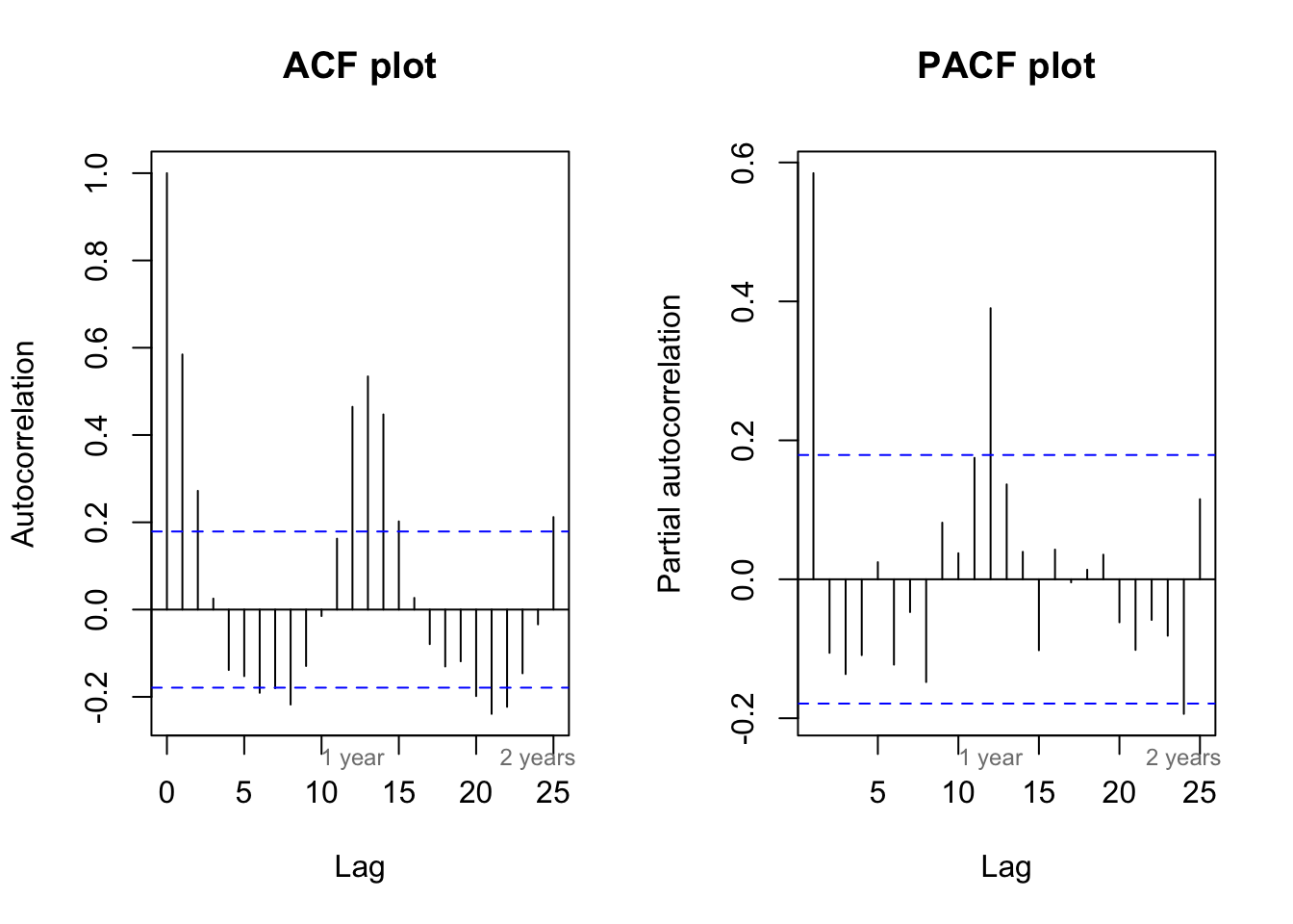

Autocorrelation structure of a seasonal timeseries

The ACF plot shows the persistence typical of an AR process, but rather than scaling geometrically down to zero, we see long-term cyclical behavior with peaks at lags 12 and 24 (1 and 2 years). The PACF plot shows the dramatic dropoff after lag 1 typical of an AR(1) process, but then a second peak at lag 12 (1 year).

Our conclusion is that this time series process can be at least weakly predicted not only by what happened last month, but also what happened last year at this time. Many real-world datasets display this type of double dependency — for example, my inspiration for this simulated data was rainfall totals. There are wet years and dry years, so knowing if the previous month’s rainfall totals were high or low is often helpful to determining whether this month’s rainfall levels were high or low \((Y_t \approx Y_{t-1})\). But there are also wet months and dry months, so knowing the rainfall levels 12 months ago is also helpful in determining this month’s rainfall levels \((Y_t \approx Y_{t-12})\).

We can model this data as a long-order AR process with nonzero coefficients at 1 and 12 lags, something like AR(0.5,0,0,0,0,0,0,0,0,0,0,0.3), but this seems (and is) unnecessarily cumbersome for a data property we expect to encounter again and again. Instead, we will find new efficiencies through the use of the backshift operator.

Definition

Note

Let \(\boldsymbol{Y}\) be a time series random variable observed at regular time periods \(T = \{1, 2, \ldots, n\}\), with a known seasonal period of \(m\). Let \(\boldsymbol{\omega}\) be a white noise process observed at the same time periods. If there exist characteristic polynomials \(\Phi(B),\varPhi_s(B^m), \Theta(B), \varTheta_s(B^m)\) with polynomial power \(p, P, q, Q\) respectively, such that the relationship between \(\boldsymbol{Y}\) and \(\boldsymbol{\omega}\) can be written:

\[Y_t \cdot \Phi(B) \cdot \varPhi_s(B^m) (1 - B)^d (1 - B^m)^D= \omega_t \cdot \Theta(B) \cdot \varTheta_s(B^m)\]

Then we say that \(\boldsymbol{Y}\) follows an seasonal autoregressive integrated moving average (SARIMA) model written SARIMA(p,d,q)(P,D,Q)_m.

That equation looks menacingly dense, so maybe we can tease it apart:

\[Y_t \cdot \Phi(B) = 1 - \phi_1Y_{t-1} - \phi_2Y_{t-2} - \ldots - \phi_pY_{t-p}\]

The first polynomial \(\Phi(B)\) describes autocorrelation between \(Y_t\) and its immediate lags.

\[Y_t \cdot \varPhi_s(B^m) = 1 - \varphi_1Y_{t-m} - \varphi_2Y_{t-2m} - \ldots - \varphi_PY_{t-Pm}\]

The second polynomial \(\varPhi_s(B)\) describes autocorrelation between \(Y_t\) and its same-season values in each prior cycle.

\[Y_t \cdot (1 - B)^d = (Y_t - Y_{t-1})(1 - B)^{d-1} \ldots = \nabla^dY_t\]

The third polynomial \((1 - B)^d\) differences the series \(d\) times to achieve stationarity.

\[Y_t \cdot (1 - B^m)^D = (Y_t - Y_{t-m})(1 - B)^{D-1} \ldots = \nabla^D_mY_t\]

The fourth polynomial \((1 - B^m)^D\) shifts the analysis to differences (or second differences, etc.) from same-period values in the past seasonal periods.¹

\[\omega_t \cdot \Theta(B) = 1 + \theta_1\omega_{t-1} + \theta_2\omega_{t-2} + \ldots + \theta_q\omega_{t-q}\]

The fifth polynomial \(\Theta(B)\) describes correlation between \(Y_t\) and the immediate prior innovations in the times series.

\[\omega_t \cdot \varTheta_s(B^m) = 1 + \vartheta_1\omega_{t-m} + \vartheta_2\omega_{t-2m} + \ldots + \vartheta_q\omega_{t-Qm}\]

The sixth polynomial \(\varTheta_s(B^m)\) describes correlation between \(Y_t\) and the same-season innovations in each prior cycle.

Examples

Hypothetical monthly series

Let’s return to our hypothetical monthly dataset. We saw the first five years above. Let’s plot the last three years, with room for forecasting:

plot(c(rep(NA,84),y[85:120]),type='l',ylab=expression(Y[t]),xlim=c(85,132),ylim=c(0,6))  
abline(v=0.5+12*(8:10),lty=2,col='#7f7f7f')
text(x=12*(7:10),y=0.1,labels=paste('Year',8:11),pos=4,col='#7f7f7f')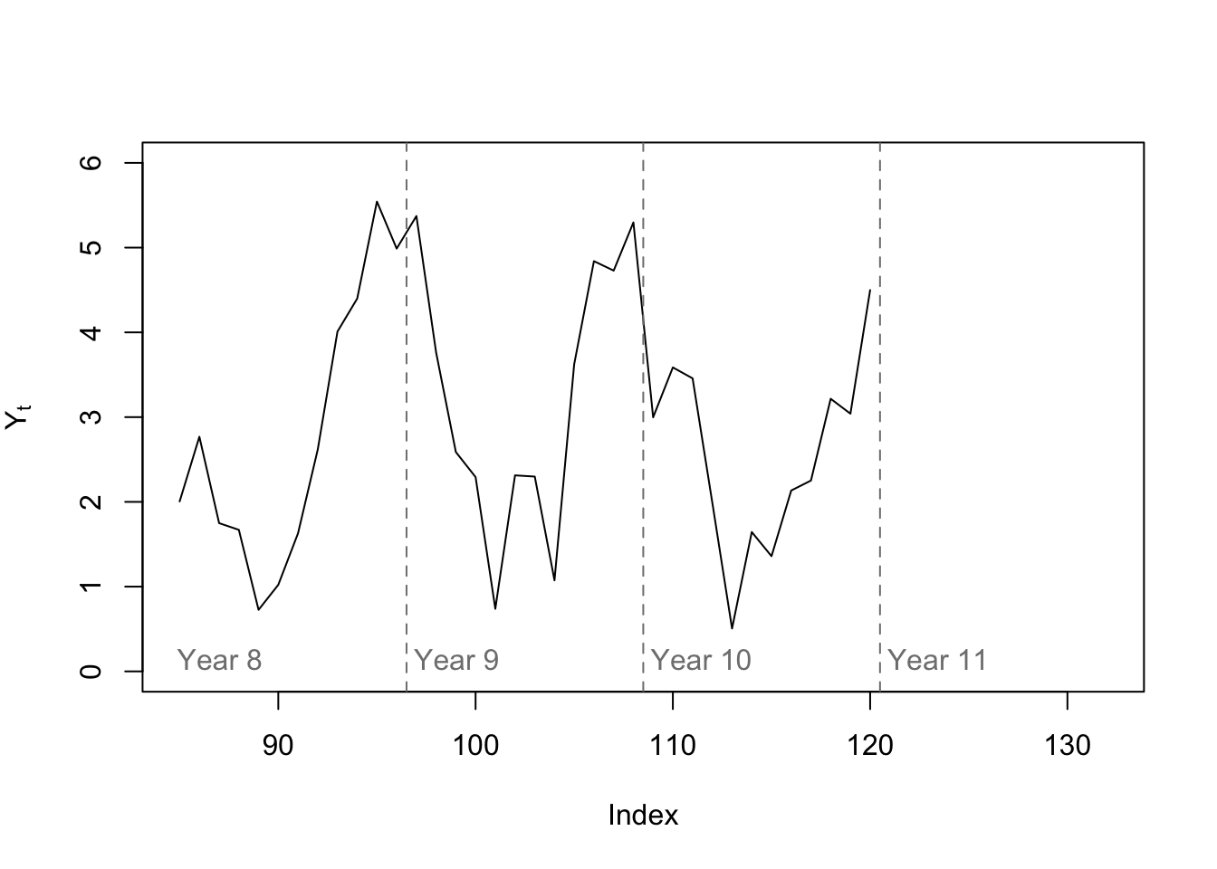

Last three years of a seasonal time series

Notice that the seasonal pattern has shifted. Instead of two peaks in spring and autumn, we now see one valley in summer and one peak in winter (this change began as early as Year 5, if you compare with the plot above). Has this wrecked the seasonality of the series? No! In a SARIMA model, all we require is that there be some correlation with the past same-season values, not that the first full period looks just like the last.

Although we could let an automated routine pick our model for us, based on the ACF and PACF plots above we might feel comfortable diagnosing a SARIMA(1,0,0)(1,0,0)₁₂:

(y.sar <- arima(y,order=c(1,0,0),seasonal=list(order=c(1,0,0),period=12)))

Call:
arima(x = y, order = c(1, 0, 0), seasonal = list(order = c(1, 0, 0), period = 12))

Coefficients:
         ar1    sar1  intercept
      0.5146  0.3706     2.5023
s.e.  0.0803  0.0897     0.2888

sigma^2 estimated as 1.06:  log likelihood = -174.84,  aic = 357.67

We can plot the forecast of this SARIMA model and, since ARIMA models are based in distributional theory and an assumption of Gaussian white noise, we can plot an 80% confidence region for our predictions:

plot(forecast(y.sar,h=12),include=36,ylab=expression(Y[t]),ylim=c(0,6),
     fcol='#0000ff',pi.col='#0000ff7f',xlab='Index')  
abline(v=0.5+12*(8:10),lty=2,col='#7f7f7f')
text(x=12*(7:10),y=0.1,labels=paste('Year',8:11),pos=4,col='#7f7f7f')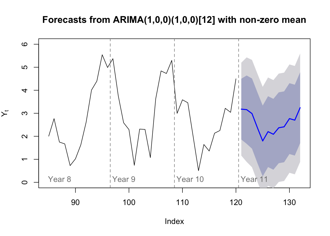

12-month lookahead forecasts from SARIMA model

Airline passengers data

We also examined this data when learning about exponential smoothing models.

plot(AirPassengers)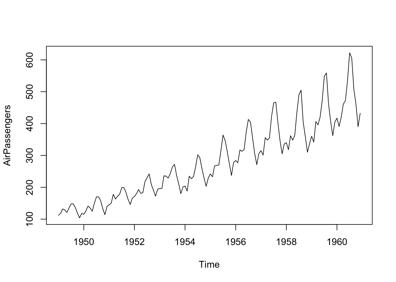

Box-Jenkins airline passenger data

The data show both clear seasonality as well as clear non-stationarity. A Box-Cox transform might help:

par(mfrow=c(1,2))
boxcox(AirPassengers~1)
title(main=expression(paste('Likelihoods for Box-Cox ',lambda)))
plot(log(AirPassengers))
title(main=expression(paste('Box-Cox transformed data, ',lambda == 0)))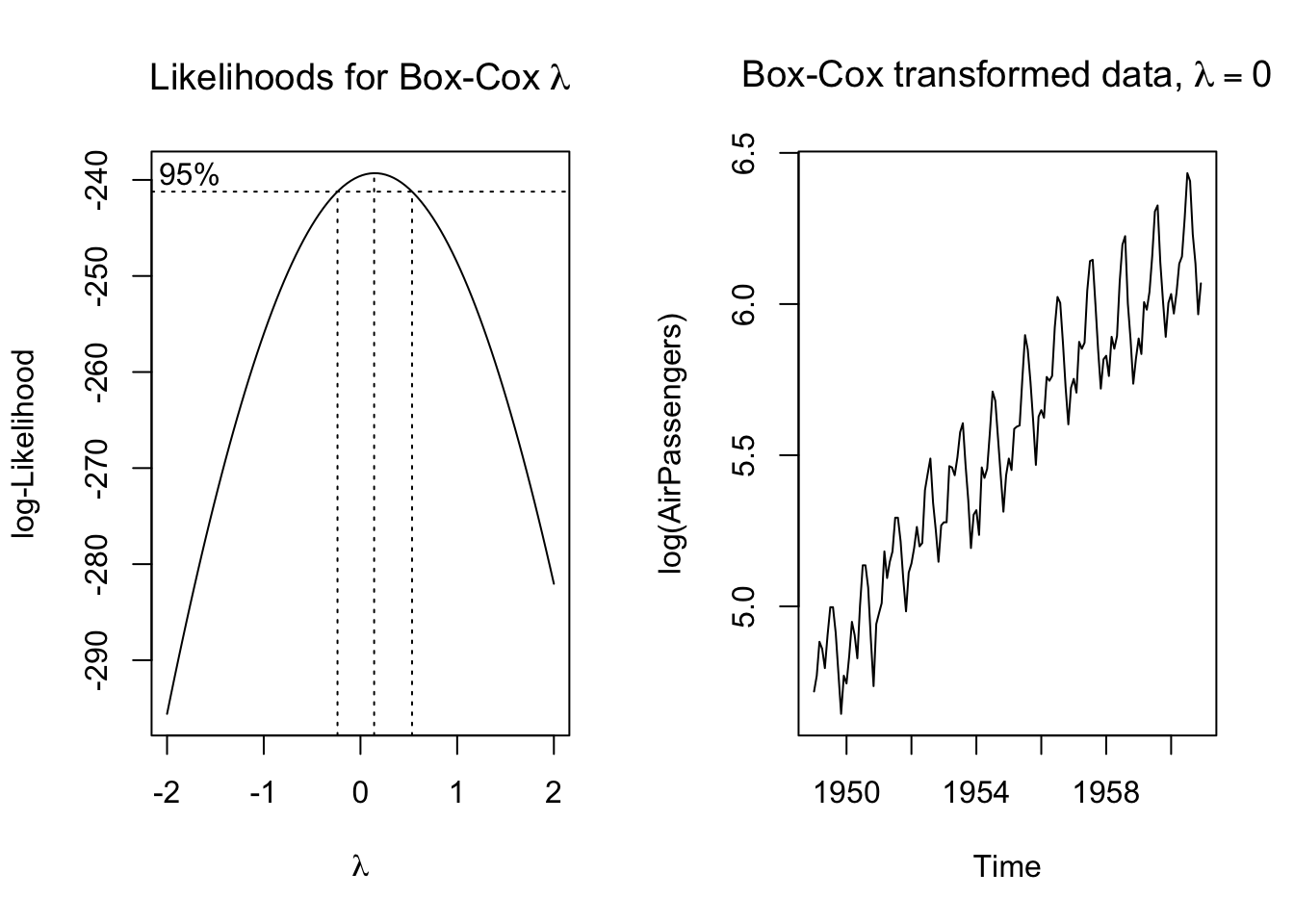

We seem to have reached trend stationarity. Tests will confirm:

suppressWarnings(adf.test(log(AirPassengers)))

    Augmented Dickey-Fuller Test

data:  log(AirPassengers)
Dickey-Fuller = -6.4215, Lag order = 5, p-value = 0.01
alternative hypothesis: stationary

suppressWarnings(kpss.test(log(AirPassengers),null='Trend'))

    KPSS Test for Trend Stationarity

data:  log(AirPassengers)
KPSS Trend = 0.11267, Truncation lag parameter = 4, p-value = 0.1

We are ready to fit a SARIMA model:

air.sarima <- auto.arima(AirPassengers,lambda=0)
summary(air.sarima)

Series: AirPassengers 
ARIMA(0,1,1)(0,1,1)[12] 
Box Cox transformation: lambda= 0 

Coefficients:
          ma1     sma1
      -0.4018  -0.5569
s.e.   0.0896   0.0731

sigma^2 = 0.001371:  log likelihood = 244.7
AIC=-483.4   AICc=-483.21   BIC=-474.77

Training set error measures:
                     ME     RMSE      MAE          MPE     MAPE     MASE
Training set 0.05140415 10.15504 7.357553 -0.004079018 2.623636 0.229706
                    ACF1
Training set -0.03689682

Notice that although the series has a clear nonzero mean and a clear deterministic trend, neither effect appears in the model summary! We will explore this more in a moment.

We see a sensible model with few parameters, each with estimates several times larger than their standard errors, which is usually comforting to a statistician. This SARIMA(0,1,1)(0,1,1)₁₂ model suggests the following:

• First, we are looking at a double-differenced model: once differenced against its first lag, and then re-differenced against its 12^th lag. The double differencing is why we do not need to estimate a mean/level or a trend/slope: the double difference of a linear trend is zero.

• Second, there are no AR terms or seasonal AR terms (somewhat surprisingly!), only MA and seasonal MA terms. Rather than creating an echoing chain of dependency across months and across years, we will simply focus on what happened last month and what happened 12 months ago.

• Third, the MA(1) term and seasonal MA(1) term are negative, meaning that we see some degree of error correction. If the innovation from last month was estimated to be extreme, then we will partially ignore it when modeling this month’s difference. If the innovation from 13 months ago was estimated to be extreme, then we will partially ignore it when constructing the year-ago monthly difference which becomes the reference point for this month’s difference.

• Fourth, consider that this model implies the following approximate equivalency: \(\log Y_t - \log Y_{t-1} \approx \log Y_{t-12} - \log Y_{t-13}\). We can re-arrange terms to say that:

\[Y_t = e^{\log Y_{t-1} + \log(Y_{t-12}/Y_{t-13})} = Y_{t-1} \times \frac{Y_{t-12}}{Y_{t-13}}\]

In other words, our model suggests that the best prediction of this month’s airline passenger volume is equal to last month’s volume, plus the prior-year proportional increase between the same two months, plus or minus some error correction which is meant to mute the effect of one-off shocks and unusually large innovations. Between a log-transform and the two types of differencing, we were able to describe a multiplicative growth and multiplicative seasonality model using a representation intended for linear, stationary time series!

---

1. Recall that \(\nabla^D\) represents the D^th-order difference, while \(\nabla_m\) represents the first-order difference between \(Y_t\) and its m^th lag \(Y_{t-m}\), so \(\nabla^D_m\) is the D^th-order difference using the m^th lag.