A second building block of statistical time series analysis is the moving average (MA) model. Moving average models are not well-named: rather than predicting \(Y_t\) as a weighted average of its past values (which is what AR models can do), MA models predict \(Y_t\) using a weighted average of the unobserved innovations:
Once again I have sketched this idea using the terminology familiar to us from linear regression, but below I will redefine this idea using our new time series notation.
MA(1) process
Let’s take the simplest case, where each value of the series averages only the current and immediate previous innovation. We would name this an moving average model with order 1 or MA(1) model.
Note
Let \(\boldsymbol{Y}\) be a time series random variable observed at regular time periods \(T = \{1, 2, \ldots, n\}\). Let \(\boldsymbol{\omega}\) be a white noise process observed at the same time periods. If,
\[Y_t = \omega_t + \theta \omega_{t-1}\]
For some \(\theta \in \mathbb{R}\) and all \(t \in T\), then we say that \(\boldsymbol{Y}\) is an moving average process with order 1
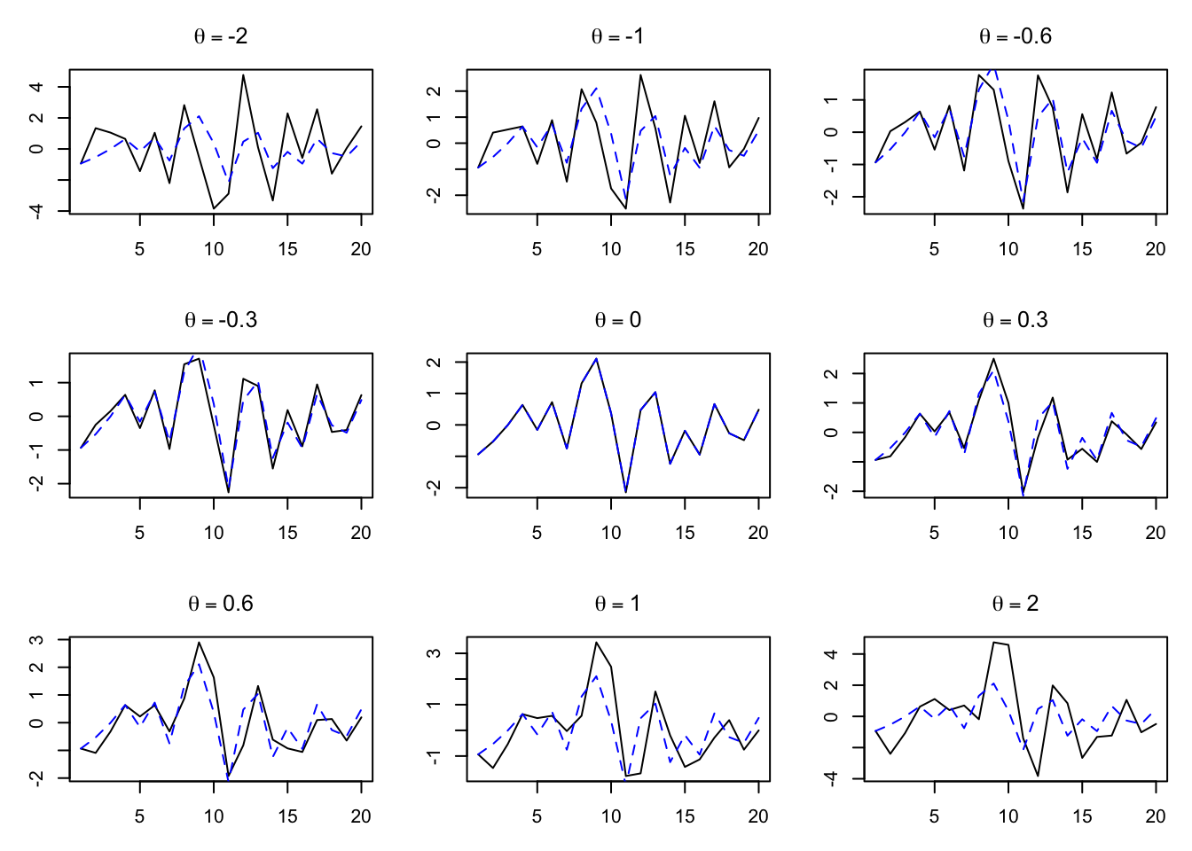
In theory, the exact properties of a MA(1) process depend on both the moving average parameter \(\theta\) as well as the specific type of white noise process denoted by \(\boldsymbol{\omega}\). In practice, we often assume \(\boldsymbol{\omega}\) to be Gaussian white noise, leaving \(\theta\) as the only input which needs estimation.
In the plots above, we see that MA processes are a little more subtle than AR processes:
MA(1) processes remain stationary for any finite value of \(\theta\), even large positive or negative values. (The weighted sum of any two zero-mean random variables still has a mean of zero.)
Positive and negative values of \(\theta\) produce similar patterns, with no parameter choice creating the alternating series seen in the AR(1) models.
The properties and utility of MA models are perhaps better described with higher-order processes.
Generalizing to MA(q)
Now we may complicate the scenario, by allowing the current value \(Y_t\) to average several, different past innovations of the series.
Note
Let \(\boldsymbol{Y}\) be a time series random variable observed at regular time periods \(T = \{1, 2, \ldots, n\}\). Let \(\boldsymbol{\omega}\) be a white noise process observed at the same time periods. If,
For some \((\theta_1, \theta_2, \ldots, \theta_q) \in \mathbb{R}^q\) and all \(t \in T\), then we say that \(\boldsymbol{Y}\) is an moving average model with orderq.
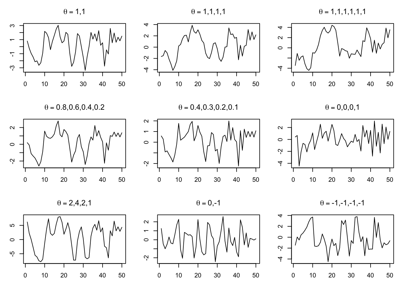
MA(q) effects tend to become more pronounced at higher orders. For many combinations of parameters \(\theta_1, \ldots, \theta_q\), the general effect is a smoothing filter which highlights consecutive large innovations but minimizes single innovations, and preserves no memory of the past beyond its averaging:
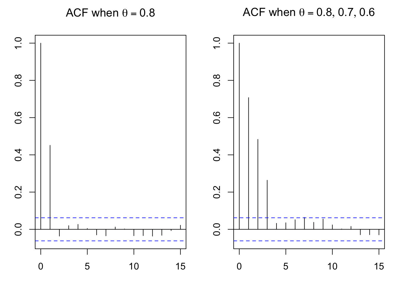
An autocorrelation function (ACF) plot will always provide helpful summary or diagnostic information about a MA(q) model. In the simplest case of MA(1), the height of the ACF plot at the first lag will be equal to \(q/(1+q^2)\), and the remaining lags will show little or no autocorrelation at all. For example, when \(\theta=0.8\), the first lag will have an autocorrelation of roughly \(0.8/(1+0.64) \approx 0.49\), and all other lags will show only minimal autocorrelation:
Code
par(mfrow=c(1,2),mar=c(3.1,3.1,3.1,1.1))set.seed(0108)ma08 <-arima.sim(list(ma=0.8),n=1000)ma080706 <-arima.sim(list(ma=c(0.8,0.7,0.6)),n=1000)acf(ma08,main=expression(paste('ACF when ',theta ==0.8)),lag.max=15)acf(ma080706,main=expression(paste('ACF when ',theta ==list(0.8,0.7,0.6))),lag.max=15)
Two MA processes and their ACF plots, 1000 obs each
The key feature here is that for values \(s \lt (t - q)\), \(Y_t\) and \(Y_s\) have no elements in common and are completely independent. Any small sample autocorrelation is purely spurious.
All MA processes are stationary
Since MA processes are simply weighted sums of zero-mean white noise, they themselves are zero-mean and meet all the requirements for weak stationarity, no matter the choice(s) of \(\boldsymbol{\theta}\). In the equations which follow, assume that \(\mathbb{E}[\omega_t] = 0\) and \(\mathbb{V}[\omega_t] = \sigma^2\):
We can see from the above that the mean and variance are constant and that the autocovariance of two entries depends only on the lag between them, which are the requirements of weak stationarity.
MA model responses to system shocks
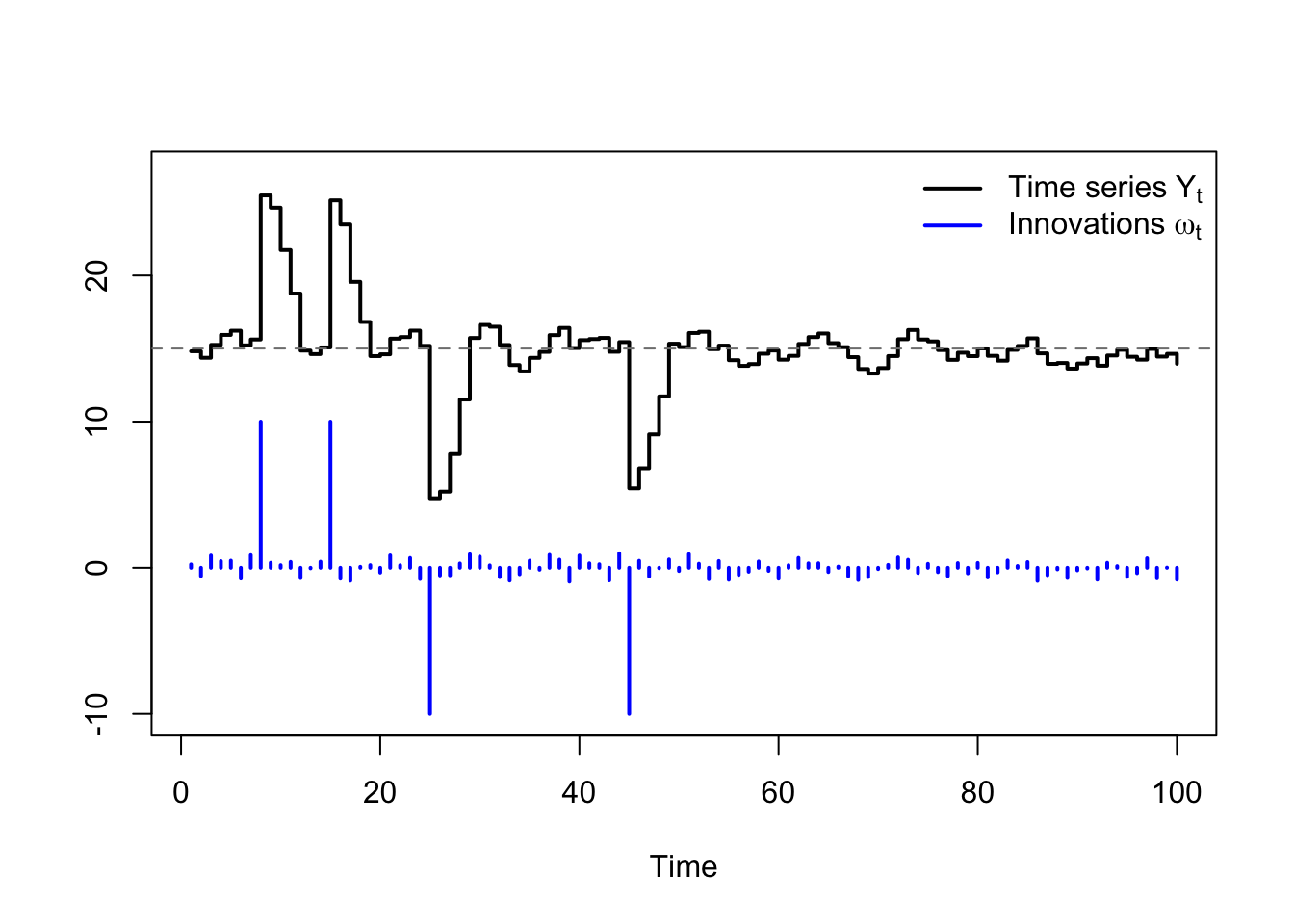
MA models dampen one-time system shocks by averaging them among the other innovations, and after the moving average window has passed, the system shock disappears entirely from the series. Consider a MA(3) model which processes a fairly quiet series of innovations, interrupted irregularly by a much larger signal: