Code
par(mfrow=c(1,2),mar=c(4, 4, 3, 1))
y1 <- sin((1:1200)*2*pi/100)
plot(y1,type='b',pch=20,xlim=c(1,200))
spectrum(y1,log='no',xlim=c(0,0.2))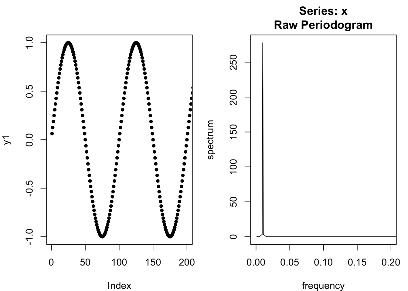
Imagine observing a signal with a strong periodicity, like a sine wave. We could depict that signal as a waveform in the time domain (the world we experience). We could also depict that signal as a peak in the frequency domain (i.e. the spectral density). Let’s suppose that the signal repeats every 100 time-units, for a frequency of 0.01:
par(mfrow=c(1,2),mar=c(4, 4, 3, 1))
y1 <- sin((1:1200)*2*pi/100)
plot(y1,type='b',pch=20,xlim=c(1,200))
spectrum(y1,log='no',xlim=c(0,0.2))
Now imagine a more complicated signal, a composite of our first signal and a new signal which repeats every 20 units, creating a new spectral density peak at 0.05:
par(mfrow=c(1,2),mar=c(4, 4, 3, 1))
y2 <- sin((1:1200)*2*pi/20)
plot(y1+y2,type='b',pch=20,xlim=c(1,200))
spectrum(y1+y2,log='no',xlim=c(0,0.2))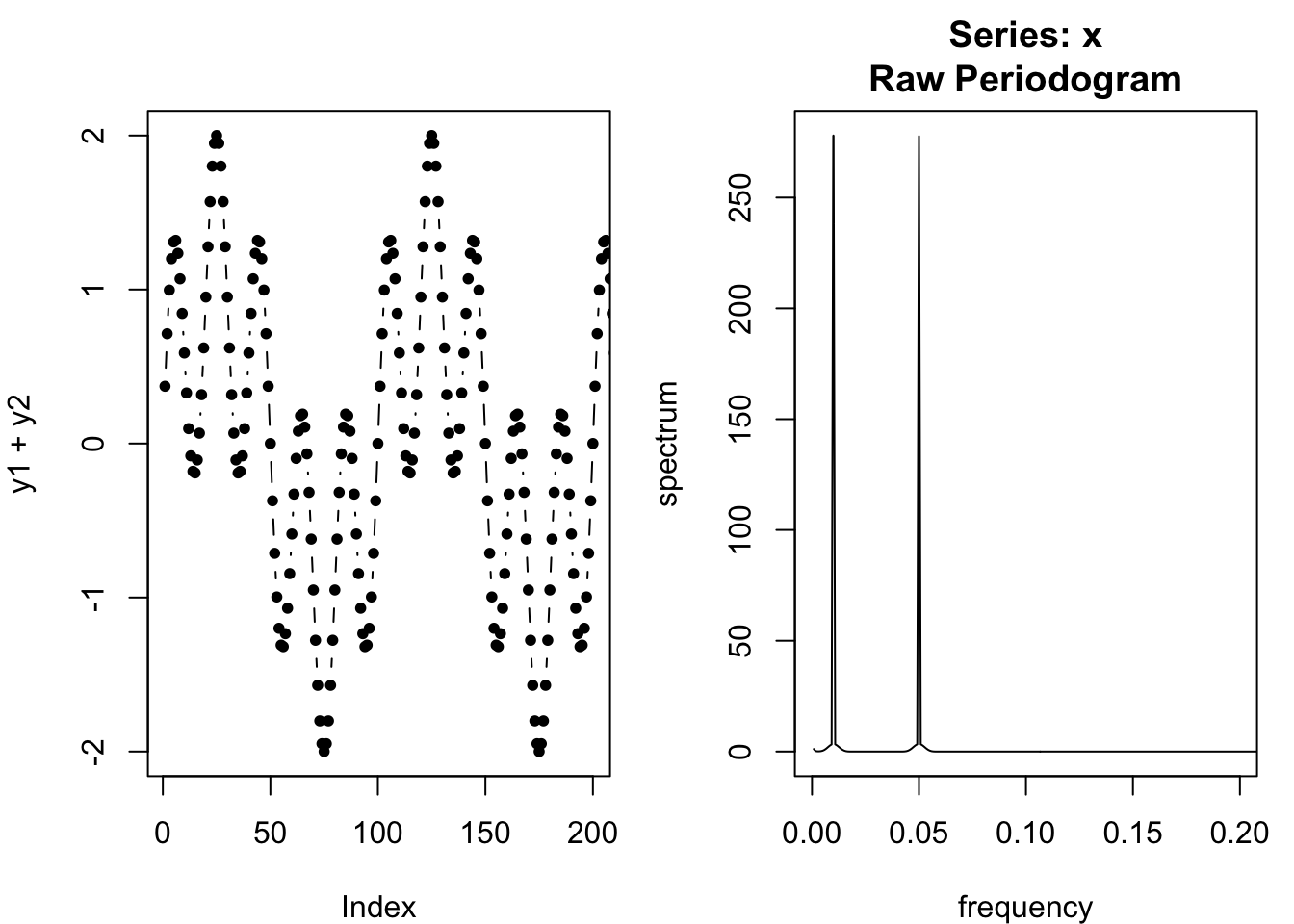
We can continue to add more peaks to the spectral density, for example by adding a new waveform with a period every 8 observations (for a frequency of 0.125):
par(mfrow=c(1,2),mar=c(4, 4, 3, 1))
y3 <- sin((1:1200)*2*pi/8)
plot(y1+y2+y3,type='b',pch=20,xlim=c(1,200))
spectrum(y1+y2+y3,log='no',xlim=c(0,0.2))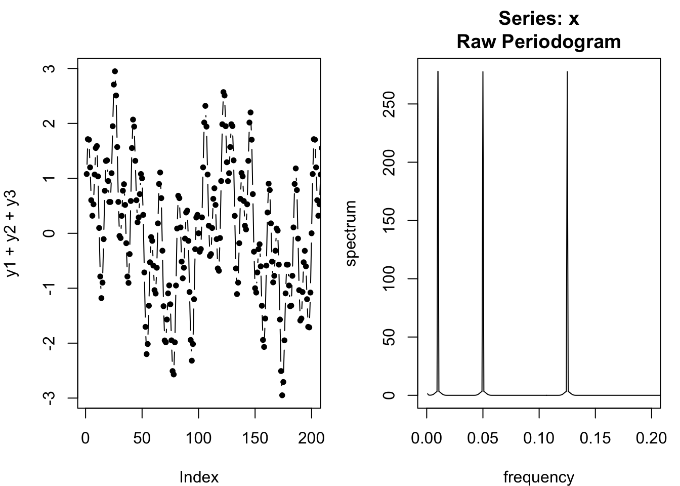
Let’s take this to the limit case: what if the spectral density were equally powerful at every frequency? We call this white noise:
par(mfrow=c(1,2),mar=c(4, 4, 3, 1))
y4 <- rnorm(100000)
plot(y4,type='b',pch=20,xlim=c(1,200))
spectrum(y4,log='no',xlim=c(0,0.2))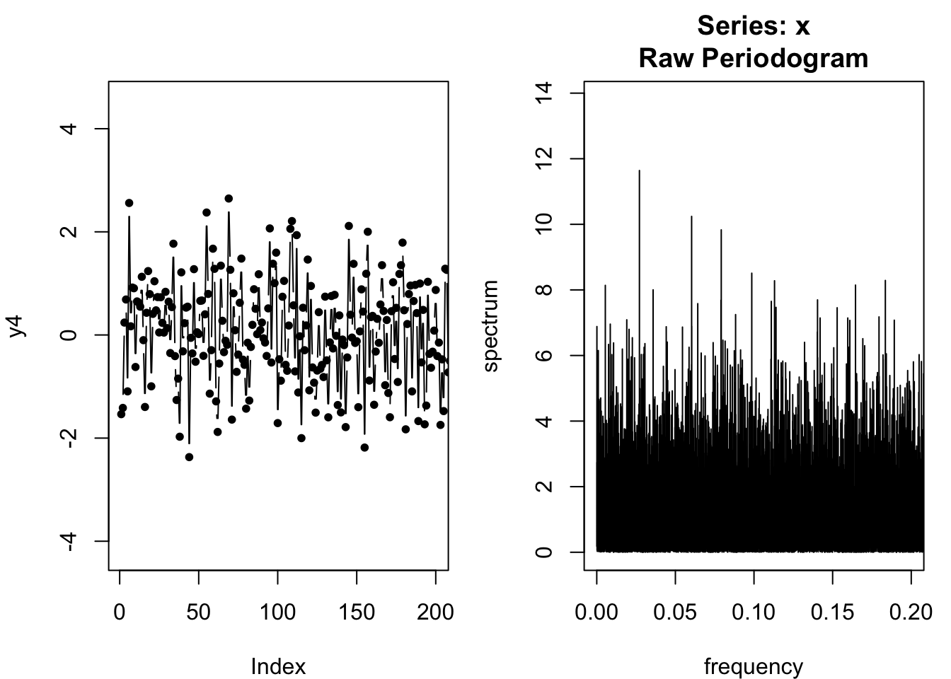
White noise refers to any time-domain generating process which has uniform power across the frequency domain. It has no connection to anyone named White1, and instead is a metaphor for “white light” — light which is equally strong across all wavelength frequencies in the visible part of the electomagnetic spectrum.
Many different series can be white noise. Choosing either -1 or +1 with equal and independent probability would be a series of white noise. White noise must have the following properties in the time domain:
The observations must show no serial correlation, and in fact most definitions require that they be statistically independent of each other.2
The observations must have mean 0.
The observations must have a finite variance.
Although many series can be white noise, some of the models we will study in this course assume that the white noise takes a specific form, where each observation is drawn from an IID Normal distribution with mean zero and constant variance. In other words, the error process we normally3 associate with a linear regression is also white noise, and is often used to describe the error process of time series models. (The Normal distribution is also called the Gaussian distribution.)
An individual value from a white noise process is sometimes called an “innovation” or a “random shock” instead of an “error”. We will generally use the term “innovation” in this course, rather than “error”, to emphasize that the shocks are not wrong or misleading in any sense, they are simply unknown until the moment they happen; they are new discoveries that change the status quo.
To reinforce this perspective, white noise innovations in a time series model are generally denoted as \(\omega_1, \omega_2, \ldots, \omega_n\) and not as \(\varepsilon_1, \varepsilon_2, \ldots, \varepsilon_n\). As a mnemonic, you could say they are “w for white noise, not e for error”.
Let \(\boldsymbol{\omega}\) be a time series random variable observed at regular time periods \(T = \{1, 2, \ldots, n\}\). If \(\omega_t \sim \textrm{Normal}(0,\sigma^2)\) for all \(t \in T\) and \(\omega_s \perp \omega_t\) for all \(s,t \in T\), then the generating process \(\boldsymbol{\omega}\) is said to be additive Gaussian white noise