Forecast strategies

So far we’ve learned about two classes of time series models: ARIMA (including variants like SARIMA), and exponential smoothing models. Both of these models describe a data generating process in which each new observation evolves from an iterative calculation dependent upon the immediate prior observation(s).

Forecasting both of these models involves “walking” or “unfolding” the process forward, one step at a time. The easiest way to understand our projection for \(\hat{y}_{t+2}\) from the information gathered at time \(t\) is to first compute our projection for \(\hat{y}_{t+1} | y_t\), and then continue to calculate \(\hat{y}_{t+2} | y_t, \hat{y}_{t+1}\).

This is a very intuitive idea, and for many datasets it produces effective results with relatively modest compute and memory requirements. In the right contexts, however, alternative strategies will outcompete these models. We will learn a little more about the different strategies available to us below.

Notation

In all of the discussion on this page, I will try to keep to the following notation, as similar as possible to what we have already been using, and as similar as possible to the discussion found in Ben Taieb, et al. (2012).

Term Meaning
\(y_1, \ldots, y_N\) The training data used to build all models
\(y_N\) The last observation in the training data
\(y_t\) Any generic observation (not necesarily the last observation)
\(\hat{y}_{N+t}\) Any generic forecasted future observation
\(f\) A conceptual model of the data generating process
\(w\) A “fudge factor” including all noise, anomalies, and modeling error
\(\hat{f}\) A “one-ahead” forecasting function, prefit using all training data
\(\hat{f_h}\) An “h-ahead” forecasting function, prefit using all training data
\(d\) The embedding dimension (how many past observations are used as forecasting inputs)
\(H\) The maximum number of periods for which a forecast is needed
\(\boldsymbol{w}\) A vectorized “fudge factor”, \(\boldsymbol{w} \in \mathbb{R}^H\)
\(F\) A multivariate model of the data generating process, \(F:\mathbb{R}^d \rightarrow \mathbb{R}^H\)
\(\hat{F}\) A multivariate forecasting function, prefit using all training data
\(I\) The number of forecasting “blocks” in a DIRMO strategy
\(s\) The size of each forecasting “block” in a DIRMO strategy

Recursive forecasting

Theory

This strategy is the first we have learned, and applies to ARIMA models, ETS models, state space models, some KNN (k-nearest neighbor) models, and some RNN (recursive neural network) models, among others.

All of these models use a data generating process which can be expressed as follows:

\[y_t = f(y_{t-d}, \ldots, y_{t-1}) + w\]

Note that the true data generating process \(f\) is not itself data-dependent. For example, if we are studying an ARMA(1,2) process, the true parameters \(\phi_1, \theta_1, \theta_2\) are fixed in stone (yet usually unknown). The data may guide us close to them or wildly mislead us, but \(\phi_1, \theta_1, \theta_2\) do not change when we observe our sample.

However, even though the nature of the function itself is not data-dependent, the specific outputs of any function depend on the inputs, and if we were again considering an ARMA(1,2) process (where \(d=2\)) we could say that \(y_t\) is a function of \(y_{t-1}\) and \(y_{t-2}\) plus some white noise, misspecification, parameter drift, etc., which we can aggregate into the error term \(w\).

Forecasting from this model involves estimating the data generating process \(f\) from the data, resulting in the forecasting function \(\hat{f}_h\) for any observation \(h\) steps into the future. The inputs to this function are all “real” observations, all “forecasts”, or a mix of the two, depending on the embedding dimension \(d\) and the forecast horizon \(h\):

\[\hat{y}_{N+h} = \left\{ \begin{array}{ll} \hat{f}(y_{N-d+1}, \ldots, y_N) & \textrm{if} \; h=1 \\ \hat{f}(y_{N-d+h}, \ldots, y_N,\hat{y}_{N+1}, \ldots, \hat{y}_{N+h-1}) & \textrm{if} \; h=2,\ldots,d \\ \hat{f}(\hat{y}_{N+h-d}, \ldots, \hat{y}_{N+h-1}) & \textrm{if} \; h \gt d \end{array} \right\}\]

Example: AR(2) model

Suppose we model a time series sample (with 100 observations) using an AR(2) process. That is, we believe the embedding dimension \(d=2\), and that:

\[\begin{aligned} y_t &= \phi_1 y_{t-1} + \phi_2 y_{t-2} + \omega_t \\ \\ &= f(y_{t-1},y_{t-2}) + w \end{aligned}\]

Using all 100 observations, we train our model and conclude that \(\phi_1 = 0.5\) and \(\phi_2 = 0.4\). This allows us to use a resursive forecast function to define forecasts for time indices 101, 102, and 103:

Code
y <- c(1.8, 2.5, 2.1, 3.0, 2.0)
yhat <-    0.5*y[5]    + 0.4*y[4]
yhat[2] <- 0.5*yhat[1] + 0.4*y[5]
yhat[3] <- 0.5*yhat[2] + 0.4*yhat[1]

plot(96:100,y,xlim=c(96,103),pch=19,type='b',xlab='Time index')
points(99:100,y[4:5],pch=0,cex=1.5,col='#ff0000',lwd=2)
points(101,yhat[1],pch=17,col='#0000ff')
legend(x='topright',legend=c('Observations','Forecasting inputs','Forecasts'),bty='n',pch=c(19,0,17),col=c('#000000','#ff0000','#0000ff'))
plot(96:100,y,xlim=c(96,103),pch=19,type='b',xlab='Time index')
points(100:101,c(y[5],yhat[1]),pch=0,cex=1.5,col='#ff0000',lwd=2)
points(101:102,yhat[1:2],pch=17,col='#0000ff')
legend(x='topright',legend=c('Observations','Forecasting inputs','Forecasts'),bty='n',pch=c(19,0,17),col=c('#000000','#ff0000','#0000ff'))
plot(96:100,y,xlim=c(96,103),pch=19,type='b',xlab='Time index')
points(101:102,yhat[1:2],pch=0,cex=1.5,col='#ff0000',lwd=2)
points(101:103,yhat[1:3],pch=17,col='#0000ff')
legend(x='topright',legend=c('Observations','Forecasting inputs','Forecasts'),bty='n',pch=c(19,0,17),col=c('#000000','#ff0000','#0000ff'))

Recursive forecast for h=1

Recursive forecast for h=2

Recursive forecast for h=3

Properties

Strengths of recursive forecasting:

  • Intuitive: For models like ARIMA and ETS, the forecasting method matches the data generation process. For all recursive forecasting, we predict by simulating an evolving world one step at a time, matching our own experience of reality.

  • Preserves time-dependency: Autocorrelations and other dependencies between observations are preserved over a multi-period forecast.

  • Lightweight: Neither the model nor the forecasting function need to be re-fit, simply re-applied in a single loop.

  • User-proof: No hyperparameters mean that nothing that can be set “wrong”.

Weaknesses of recursive forecasting:

  • Compounding errors: Small errors in each period’s forecast usually aggregate and get fixed into future-period forecasting, dragging later forecasts far from their actual values.

  • Strong assumptions: Recursive models imply that the data generating process is constant (or at least similarly parameterized) throughout the past and future. They are less effective in the face of mixture models, high volatility, structural breaks, etc.

Direct forecasting

Theory

Rather than understanding future time period \(N+2\) as a function of the current time period \(N\) and the next time period \(N+1\), we could simply create a new forecasting function \(\hat{f_2}\) custom-built for two-ahead prediction. This new forecasting function would not need the prediction \(\hat{y}_{N+1}\) as an input.

This forecasting method matches well with neural networks, some KNN models, and many series displaying weak time-series behavior which might otherwise be modeled with time-invariant techniques such as regression.

Even if the “true” data generating process evolves iteratively, direct forecasting strategies believe that each observation \(y_t\) can be usefully modeled by several different functions, each of which use a different set of prior values:

\[\begin{aligned} y_t &= f_1(y_{t-d}, \ldots, y_{t-1}) + w \\ y_t &= f_2(y_{t-d-1}, \ldots, y_{t-2}) + w \\ \vdots & \\ y_t &= f_H(y_{t-d-H+1}, \ldots, y_{t-H}) + w \end{aligned}\]

This structure allows us to estimate a set of forecasting functions, which use only observed values \(y_t\) as inputs:

\[\hat{y}_{N+h} = \hat{f_h}(y_{N-d+1}, \ldots, y_N)\]

Example: Non-exponential smoothing

Suppose an economist is making predictions about future inflation rates. They know that inflation has averaged 2% per annum over the last several decades, and they also know that, in the short-term, the inflation rate this quarter is a good predictor of the inflation next quarter. They devise the following forecast models:

\[\begin{aligned} \hat{y}_{N+1} = {f_1}(y_N) = 0.8y_N + 0.2(0.02) \\ \hat{y}_{N+2} = {f_2}(y_N) = 0.6y_N + 0.4(0.02) \\ \hat{y}_{N+3} = {f_3}(y_N) = 0.4y_N + 0.6(0.02) \\ \hat{y}_{N+4} = {f_4}(y_N) = 0.2y_N + 0.8(0.02) \end{aligned}\]

(Implicitly, we might add that \(\hat{y}_{N+h} = 0.02\) for any \(h \gt 4\)). This model shows a mean reversion from the current value which could also be modeled with an AR(1) process; however, the AR decay is exponential and our economist may have empirical evidence to suggest that inflation rates revert to the mean at a steadier pace.

Code
y <- c(0.025, 0.021, 0.02, 0.03)
yhat <- c(0.8,0.6,0.4,0.2)*y[4] + c(0.2,0.4,0.6,0.8)*0.02

plot(1:4,y,xlim=c(1,8),pch=19,type='b',xlab='Quarter',ylab='Inflation rate',xaxt='n')
axis(side=1,at=1:8,labels=c(paste0('2025Q',1:4),paste0('2026Q',1:4)))
points(4,y[4],pch=0,cex=1.5,col='#ff0000',lwd=2)
points(5:8,yhat,pch=17,col='#0000ff')
legend(x='topleft',legend=c('Observations','Forecasting inputs','Forecasts'),bty='n',pch=c(19,0,17),col=c('#000000','#ff0000','#0000ff'))

Direct forecasts for h=1,2,3,4

Properties

Strengths of direct forecasting:

  • Robust: By fitting separate models for each time horizon, we stop large errors in one forecast from contaminating future-period forecasts.

  • Only uses observed data: Conceptually, these models do not need any “guesses” about an intermediate future state in order to make their forecasts.

  • Resource needs independent of forecast horizon: Generally, a forecast for time \(N+100\) requires the same amount of resources as the forecast for time \(N+1\), unlike recursive models which must simulate 99 additional steps.

Weaknesses of direct forecasting:

  • Erases interdependence between forecast values: The forecasts are all conditionally independent of each other, and so direct forecasts for adjacent time periods might suggest improbable or nonsensical single-period changes, or ignore useful information from intermediate forecast periods.

  • More resource-intensive: Separate models must be trained and stored for each forecast horizon.

Multiple-input multiple-output (MIMO) forecasting

Theory

Both of the strategies described above forecast a single future period; that is, each forecasting model \(\hat{f}\) or \(\hat{f_h}\) is a real-valued function of one or more inputs which produces one output, our forecast \(\hat{y}_{N+h}\).

One tension between these two strategies is that recursive forecasts understands the interdependency between different forecast points, but is prone to accumulate and amplify forecasting error. Contrariwise, direct forecasting avoids the compounding errors by destroying the links between forecasted values.

Multiple-input multiple-output (MIMO) forecasting attempts to resolve this tension by forecasting all future periods within the time horizon \(H\) at once. No matter how the current values of the series evolved, any subset of \(H\) observations can be usefully modeled en masse by the \(d\) prior values:

\[(y_{t-H+1}, \ldots, y_t) = F(y_{t-d-H+1}, \ldots, y_{t-H}) + \boldsymbol{w}\]

This structure allows us to estimate a multivariate forecasting function which will allow us to predict the entire forecasting horizon at once:

\[(\hat{y}_{N+1}, \ldots, \hat{y}_{N+h}) = \hat{F}(y_{N-d+1}, \ldots, y_N)\]

The outputs of these models can display correlations and other dependencies (like recursive forecasting), while imposing set-level constraints which discourage one unusual forecast from unduly influencing the other forecasts.

These forecasting strategies appear commonly in transformer-based architectures, which seek to predict the next several tokens/events at the same time, using a shared representation space for all of the tokens/events. MIMO strategies also do very well in probabilistic forecasting, which does not seek to predict the future mean of a series, but instead allows for probabilistic statements about how likely certain combinations of future events will be.

Example: Transit state-space modeling

Suppose a bus route through town is served by five buses. The bus route is a circuit which takes roughly 50 minutes to complete, and so the average wait time for a bus at any given stop is roughly 10 minutes.

We could try to predict the arrival time for the next few buses at any given stop from the arrival times of the prior buses at that same stop. Our knowledge of the real world constraints and goals of the bus drivers can help us model complex behavior:

  • If the last arrival time \(y_t\) was five minutes ago, the next one would be expected in five minutes and the one after that in fifteen minutes (ten minutes more).

  • If the last arrival time \(y_t\) was fifteen minutes ago, the next one is probably due very soon, and the one after that is also due very soon (bunching.)

  • Five buses should make a stop within roughly 50 minutes of the most recent bus stop.

This behavior can be well-approximated using a state space model, which we will learn about later. Given this setup, we would do well to forecast the next five bus stops from the times of the previous five bus stops:

\[(\hat{y}_{N+1}, \ldots, \hat{y}_{N+5}) = \hat{F}(\hat{y}_{N-4}, \ldots, \hat{y}_{N})\]

Code
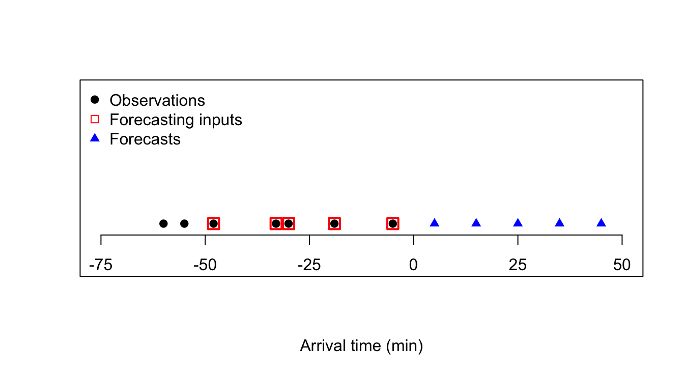
y <- c(-60,-55,-48,-33,-30,-19,-5)
yhat <- c(5,15,25,35,45)

plot(y,rep(0,7),xlim=c(-75,50),pch=19,type='p',xlab='Arrival time (min)',ylab=NA,yaxt='n',xaxt='n',ylim=c(-1,3))
axis(side=1,at=seq(-75,50,25),labels=TRUE,pos=-0.25)
points(y[3:7],rep(0,5),pch=0,cex=1.5,col='#ff0000',lwd=2)
points(yhat,rep(0,5),pch=17,col='#0000ff')
legend(x='topleft',legend=c('Observations','Forecasting inputs','Forecasts'),bty='n',pch=c(19,0,17),col=c('#000000','#ff0000','#0000ff'))
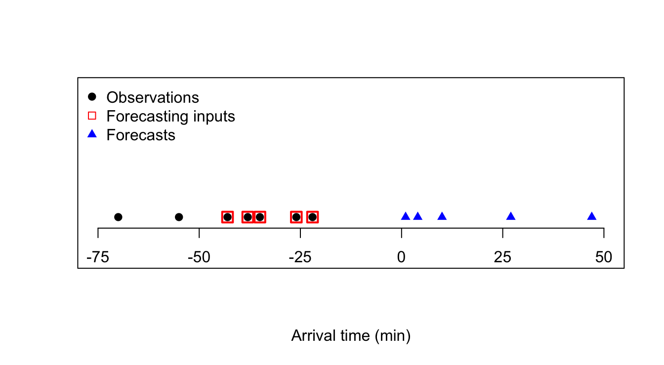
y <- c(-70,-55,-43,-38,-35,-26,-22)
yhat <- c(1,4,10,27,47)

plot(y,rep(0,7),xlim=c(-75,50),pch=19,type='p',xlab='Arrival time (min)',ylab=NA,yaxt='n',xaxt='n',ylim=c(-1,3))
axis(side=1,at=seq(-75,50,25),labels=TRUE,pos=-0.25)
points(y[3:7],rep(0,5),pch=0,cex=1.5,col='#ff0000',lwd=2)
points(yhat,rep(0,5),pch=17,col='#0000ff')
legend(x='topleft',legend=c('Observations','Forecasting inputs','Forecasts'),bty='n',pch=c(19,0,17),col=c('#000000','#ff0000','#0000ff'))

MIMO forecasts for one set of bus arrivals

MIMO forecasts for a second set of bus arrivals

Properties

Strengths of MIMO forecasting:

  • Safely handles complexity: Can learn and replicate intricate dependencies between the forecasts without compounding errors.

  • Only uses observed data: Conceptually, these models do not need any “guesses” about an intermediate future state in order to make their forecasts.

Weaknesses of MIMO forecasting:

  • Imposes one model across entire forecast period: For large values of \(H\) (the maximum forecast period), MIMO methods force a single function (or state space, or “worldview”) to describe the whole forecast range. Long-term forecasts are allowed to differ from near-term forecasts, but they must both arise from the same model.

  • Heavily resource-intensive: Multivariate outputs usually require more estimation and more compute/memory resources.

  • Burns through training data quickly: Relatedly, these models do not converge quickly and often require large amounts of data for effective accuracy, especially for large values of \(d\) and/or \(H\).

Hybrid strategies

Forecasters have explored techniques which combine these three strategies, with the goal of preserving the strengths of each stratgy while mitigating the weaknesses.

DirRec

One of these hybrids is called “DirRec” (Direct + Recursive), which outperforms both direct and recursive strategies on some real-world datasets — which should immediately raise suspicions of selection bias, confirmation bias, and publication bias.

In DirRec forecasting, each future period \(h\) is modeled with a separate function (similar to direct forecasting), but the inputs to later forecast periods include the estimated forecasts from earlier periods (similar to recursive forecasting). In other words, observations from the series can be represented as outputs from several possible generating functions, each incorporating more and more lags:

\[\begin{aligned} y_t &= f_1(y_{t-d}, \ldots, y_{t-1}) + w \\ y_t &= f_2(y_{t-d-1}, \ldots, y_{t-1}) + w \\ \vdots & \\ y_t &= f_H(y_{t-d-H+1}, \ldots, y_{t-1}) + w \end{aligned}\]

Which in turn suggest forecasting functions which need to be defined and estimated iteratively:

\[\hat{y}_{N+h} = \left\{ \begin{array}{ll} \hat{f_1}(y_{N-d+1}, \ldots, y_N) & \textrm{if} \; h=1 \\ \hat{f_h}(y_{N-d+1}, \ldots, y_N,\hat{y}_{N+1}, \ldots, \hat{y}_{N+h-1}) & \textrm{if} \; 2 \le h \le H \end{array} \right\}\]

Strengths of DirRec forecasting:

  • Implicit dependency between forecasts: Although each forecast period is modeled with a separate function, which removes explicit recursive dependencies, the presence of early forecasts among the inputs to later forecasts allows the forecasting model to re-learn those dependencies.

  • Sensible constraints on forecast outputs: The use of forecasted values as inputs can propagate errors, but since each period’s forecast function is trained separately, extreme forecasts arising from compounded errors are usually penalized and avoided.

Weaknesses of DirRec forecasting:

  • Heavily resource-intensive: To make a set of \(1 - H\)-step ahead forecasts, we must train \(H\) different models, and the later models require earlier model outputs as their inputs, complicating and lengthening the training process.

  • Loss-minimizing, not truth-seeking: Rather than seeking to parametrically understand and describe the linkages between forecast periods, DirRec locally approximates each transition.

DIRMO

A second hybrid is called “DIRMO” (Direct + Multiple Output), which establishes a spectrum of models bounded by the direct and MIMO approaches described above.

In MIMO forecasting we modeled the entire horizon of \(h \in \{1, \ldots, H\}\) with a single multivariate forecasting function \(\hat{F}\). In DIRMO forecasting, we instead split the horizon into \(I\) blocks, each of size \(s: 1 \le s \le H\). The future observations in each of these blocks will be forecasted with a separate forecasting function:

\[\begin{aligned} (\hat{y}_{N+1}, \ldots, \hat{y}_{N+s}) &= \hat{F_1}(y_{N-d+1}, \ldots, y_N) \\ &\vdots \\ (\hat{y}_{N+s(i-1)+1}, \ldots, \hat{y}_{N+si}) &= \hat{F_i}(y_{N-d+1}, \ldots, y_N) \\ &\vdots \\ (\hat{y}_{N+H-s+1}, \ldots, \hat{y}_{N+H}) &= \hat{F_I}(y_{N-d+1}, \ldots, y_N) \end{aligned}\]

Where for each \(i \in \{1, \ldots, I\}\), the forecast function \(\hat{F_i}: \mathbb{R}^d \rightarrow \mathbb{R}^s\).

Note two important edge cases. When \(s=H\), then we have only a single forecasting function, and return to MIMO forecasting. When \(s=1\), then each forecasting function returns only a single output, and we have returned to direct forecasting.

Strengths of DIRMO forecasting:

  • Loses nothing: The framework above could collapse to either MIMO or direct forcasting if and when those techniques fit the data best, or it could suggest a new approach at an optimal balance point between the two techniques.

  • Allows the far future to differ mechanically from the near future: By breaking the MIMO horizon into blocks, we allow the rules which govern far-future blocks to be different than those which estimate the near-future blocks.

Weaknesses of DIRMO forecasting:

  • Heavily resource-intensive: We now need to estimate multiple multivariate functions, and in fact will need to repeat this many times if we are optimizing the choice of block size \(s\).

  • Parameter-dependent The block size \(s\) will affect our explanatory power and model metrics, and different datasets will benefit from different sizes of \(s\) in ways which can’t easily be predicted and will be subject to overfitting when estimated from our dataset.